Statistics Tutorial
Descriptive statistics, inferential statistics, stat reference, statistics - hypothesis testing.
Hypothesis testing is a formal way of checking if a hypothesis about a population is true or not.

Hypothesis Testing
A hypothesis is a claim about a population parameter .
A hypothesis test is a formal procedure to check if a hypothesis is true or not.
Examples of claims that can be checked:
The average height of people in Denmark is more than 170 cm.
The share of left handed people in Australia is not 10%.
The average income of dentists is less the average income of lawyers.
The Null and Alternative Hypothesis
Hypothesis testing is based on making two different claims about a population parameter.
The null hypothesis (\(H_{0} \)) and the alternative hypothesis (\(H_{1}\)) are the claims.
The two claims needs to be mutually exclusive , meaning only one of them can be true.
The alternative hypothesis is typically what we are trying to prove.
For example, we want to check the following claim:
"The average height of people in Denmark is more than 170 cm."
In this case, the parameter is the average height of people in Denmark (\(\mu\)).
The null and alternative hypothesis would be:
Null hypothesis : The average height of people in Denmark is 170 cm.
Alternative hypothesis : The average height of people in Denmark is more than 170 cm.
The claims are often expressed with symbols like this:
\(H_{0}\): \(\mu = 170 \: cm \)
\(H_{1}\): \(\mu > 170 \: cm \)
If the data supports the alternative hypothesis, we reject the null hypothesis and accept the alternative hypothesis.
If the data does not support the alternative hypothesis, we keep the null hypothesis.
Note: The alternative hypothesis is also referred to as (\(H_{A} \)).
The Significance Level
The significance level (\(\alpha\)) is the uncertainty we accept when rejecting the null hypothesis in the hypothesis test.
The significance level is a percentage probability of accidentally making the wrong conclusion.
Typical significance levels are:
- \(\alpha = 0.1\) (10%)
- \(\alpha = 0.05\) (5%)
- \(\alpha = 0.01\) (1%)
A lower significance level means that the evidence in the data needs to be stronger to reject the null hypothesis.
There is no "correct" significance level - it only states the uncertainty of the conclusion.
Note: A 5% significance level means that when we reject a null hypothesis:
We expect to reject a true null hypothesis 5 out of 100 times.
Advertisement
The Test Statistic
The test statistic is used to decide the outcome of the hypothesis test.
The test statistic is a standardized value calculated from the sample.
Standardization means converting a statistic to a well known probability distribution .
The type of probability distribution depends on the type of test.
Common examples are:
- Standard Normal Distribution (Z): used for Testing Population Proportions
- Student's T-Distribution (T): used for Testing Population Means
Note: You will learn how to calculate the test statistic for each type of test in the following chapters.
The Critical Value and P-Value Approach
There are two main approaches used for hypothesis tests:
- The critical value approach compares the test statistic with the critical value of the significance level.
- The p-value approach compares the p-value of the test statistic and with the significance level.
The Critical Value Approach
The critical value approach checks if the test statistic is in the rejection region .
The rejection region is an area of probability in the tails of the distribution.
The size of the rejection region is decided by the significance level (\(\alpha\)).
The value that separates the rejection region from the rest is called the critical value .
Here is a graphical illustration:
If the test statistic is inside this rejection region, the null hypothesis is rejected .
For example, if the test statistic is 2.3 and the critical value is 2 for a significance level (\(\alpha = 0.05\)):
We reject the null hypothesis (\(H_{0} \)) at 0.05 significance level (\(\alpha\))
The P-Value Approach
The p-value approach checks if the p-value of the test statistic is smaller than the significance level (\(\alpha\)).
The p-value of the test statistic is the area of probability in the tails of the distribution from the value of the test statistic.
If the p-value is smaller than the significance level, the null hypothesis is rejected .
The p-value directly tells us the lowest significance level where we can reject the null hypothesis.
For example, if the p-value is 0.03:
We reject the null hypothesis (\(H_{0} \)) at a 0.05 significance level (\(\alpha\))
We keep the null hypothesis (\(H_{0}\)) at a 0.01 significance level (\(\alpha\))
Note: The two approaches are only different in how they present the conclusion.
Steps for a Hypothesis Test
The following steps are used for a hypothesis test:
- Check the conditions
- Define the claims
- Decide the significance level
- Calculate the test statistic
One condition is that the sample is randomly selected from the population.
The other conditions depends on what type of parameter you are testing the hypothesis for.
Common parameters to test hypotheses are:
- Proportions (for qualitative data)
- Mean values (for numerical data)
You will learn the steps for both types in the following pages.

COLOR PICKER

Contact Sales
If you want to use W3Schools services as an educational institution, team or enterprise, send us an e-mail: [email protected]
Report Error
If you want to report an error, or if you want to make a suggestion, send us an e-mail: [email protected]
Top Tutorials
Top references, top examples, get certified.

Statistics Made Easy
Introduction to Hypothesis Testing
A statistical hypothesis is an assumption about a population parameter .
For example, we may assume that the mean height of a male in the U.S. is 70 inches.
The assumption about the height is the statistical hypothesis and the true mean height of a male in the U.S. is the population parameter .
A hypothesis test is a formal statistical test we use to reject or fail to reject a statistical hypothesis.
The Two Types of Statistical Hypotheses
To test whether a statistical hypothesis about a population parameter is true, we obtain a random sample from the population and perform a hypothesis test on the sample data.
There are two types of statistical hypotheses:
The null hypothesis , denoted as H 0 , is the hypothesis that the sample data occurs purely from chance.
The alternative hypothesis , denoted as H 1 or H a , is the hypothesis that the sample data is influenced by some non-random cause.
Hypothesis Tests
A hypothesis test consists of five steps:
1. State the hypotheses.
State the null and alternative hypotheses. These two hypotheses need to be mutually exclusive, so if one is true then the other must be false.
2. Determine a significance level to use for the hypothesis.
Decide on a significance level. Common choices are .01, .05, and .1.
3. Find the test statistic.
Find the test statistic and the corresponding p-value. Often we are analyzing a population mean or proportion and the general formula to find the test statistic is: (sample statistic – population parameter) / (standard deviation of statistic)
4. Reject or fail to reject the null hypothesis.
Using the test statistic or the p-value, determine if you can reject or fail to reject the null hypothesis based on the significance level.
The p-value tells us the strength of evidence in support of a null hypothesis. If the p-value is less than the significance level, we reject the null hypothesis.
5. Interpret the results.
Interpret the results of the hypothesis test in the context of the question being asked.
The Two Types of Decision Errors
There are two types of decision errors that one can make when doing a hypothesis test:
Type I error: You reject the null hypothesis when it is actually true. The probability of committing a Type I error is equal to the significance level, often called alpha , and denoted as α.
Type II error: You fail to reject the null hypothesis when it is actually false. The probability of committing a Type II error is called the Power of the test or Beta , denoted as β.
One-Tailed and Two-Tailed Tests
A statistical hypothesis can be one-tailed or two-tailed.
A one-tailed hypothesis involves making a “greater than” or “less than ” statement.
For example, suppose we assume the mean height of a male in the U.S. is greater than or equal to 70 inches. The null hypothesis would be H0: µ ≥ 70 inches and the alternative hypothesis would be Ha: µ < 70 inches.
A two-tailed hypothesis involves making an “equal to” or “not equal to” statement.
For example, suppose we assume the mean height of a male in the U.S. is equal to 70 inches. The null hypothesis would be H0: µ = 70 inches and the alternative hypothesis would be Ha: µ ≠ 70 inches.
Note: The “equal” sign is always included in the null hypothesis, whether it is =, ≥, or ≤.
Related: What is a Directional Hypothesis?
Types of Hypothesis Tests
There are many different types of hypothesis tests you can perform depending on the type of data you’re working with and the goal of your analysis.
The following tutorials provide an explanation of the most common types of hypothesis tests:
Introduction to the One Sample t-test Introduction to the Two Sample t-test Introduction to the Paired Samples t-test Introduction to the One Proportion Z-Test Introduction to the Two Proportion Z-Test
Featured Posts
Hey there. My name is Zach Bobbitt. I have a Masters of Science degree in Applied Statistics and I’ve worked on machine learning algorithms for professional businesses in both healthcare and retail. I’m passionate about statistics, machine learning, and data visualization and I created Statology to be a resource for both students and teachers alike. My goal with this site is to help you learn statistics through using simple terms, plenty of real-world examples, and helpful illustrations.
Leave a Reply Cancel reply
Your email address will not be published. Required fields are marked *
Join the Statology Community
Sign up to receive Statology's exclusive study resource: 100 practice problems with step-by-step solutions. Plus, get our latest insights, tutorials, and data analysis tips straight to your inbox!
By subscribing you accept Statology's Privacy Policy.
- Skip to secondary menu
- Skip to main content
- Skip to primary sidebar
Statistics By Jim
Making statistics intuitive
Hypothesis Testing: Uses, Steps & Example
By Jim Frost 4 Comments
What is Hypothesis Testing?
Hypothesis testing in statistics uses sample data to infer the properties of a whole population . These tests determine whether a random sample provides sufficient evidence to conclude an effect or relationship exists in the population. Researchers use them to help separate genuine population-level effects from false effects that random chance can create in samples. These methods are also known as significance testing.

For example, researchers are testing a new medication to see if it lowers blood pressure. They compare a group taking the drug to a control group taking a placebo. If their hypothesis test results are statistically significant, the medication’s effect of lowering blood pressure likely exists in the broader population, not just the sample studied.
Using Hypothesis Tests
A hypothesis test evaluates two mutually exclusive statements about a population to determine which statement the sample data best supports. These two statements are called the null hypothesis and the alternative hypothesis . The following are typical examples:
- Null Hypothesis : The effect does not exist in the population.
- Alternative Hypothesis : The effect does exist in the population.
Hypothesis testing accounts for the inherent uncertainty of using a sample to draw conclusions about a population, which reduces the chances of false discoveries. These procedures determine whether the sample data are sufficiently inconsistent with the null hypothesis that you can reject it. If you can reject the null, your data favor the alternative statement that an effect exists in the population.
Statistical significance in hypothesis testing indicates that an effect you see in sample data also likely exists in the population after accounting for random sampling error , variability, and sample size. Your results are statistically significant when the p-value is less than your significance level or, equivalently, when your confidence interval excludes the null hypothesis value.
Conversely, non-significant results indicate that despite an apparent sample effect, you can’t be sure it exists in the population. It could be chance variation in the sample and not a genuine effect.
Learn more about Failing to Reject the Null .
5 Steps of Significance Testing
Hypothesis testing involves five key steps, each critical to validating a research hypothesis using statistical methods:
- Formulate the Hypotheses : Write your research hypotheses as a null hypothesis (H 0 ) and an alternative hypothesis (H A ).
- Data Collection : Gather data specifically aimed at testing the hypothesis.
- Conduct A Test : Use a suitable statistical test to analyze your data.
- Make a Decision : Based on the statistical test results, decide whether to reject the null hypothesis or fail to reject it.
- Report the Results : Summarize and present the outcomes in your report’s results and discussion sections.
While the specifics of these steps can vary depending on the research context and the data type, the fundamental process of hypothesis testing remains consistent across different studies.
Let’s work through these steps in an example!
Hypothesis Testing Example
Researchers want to determine if a new educational program improves student performance on standardized tests. They randomly assign 30 students to a control group , which follows the standard curriculum, and another 30 students to a treatment group, which participates in the new educational program. After a semester, they compare the test scores of both groups.
Download the CSV data file to perform the hypothesis testing yourself: Hypothesis_Testing .
The researchers write their hypotheses. These statements apply to the population, so they use the mu (μ) symbol for the population mean parameter .
- Null Hypothesis (H 0 ) : The population means of the test scores for the two groups are equal (μ 1 = μ 2 ).
- Alternative Hypothesis (H A ) : The population means of the test scores for the two groups are unequal (μ 1 ≠ μ 2 ).
Choosing the correct hypothesis test depends on attributes such as data type and number of groups. Because they’re using continuous data and comparing two means, the researchers use a 2-sample t-test .
Here are the results.

The treatment group’s mean is 58.70, compared to the control group’s mean of 48.12. The mean difference is 10.67 points. Use the test’s p-value and significance level to determine whether this difference is likely a product of random fluctuation in the sample or a genuine population effect.
Because the p-value (0.000) is less than the standard significance level of 0.05, the results are statistically significant, and we can reject the null hypothesis. The sample data provides sufficient evidence to conclude that the new program’s effect exists in the population.
Limitations
Hypothesis testing improves your effectiveness in making data-driven decisions. However, it is not 100% accurate because random samples occasionally produce fluky results. Hypothesis tests have two types of errors, both relating to drawing incorrect conclusions.
- Type I error: The test rejects a true null hypothesis—a false positive.
- Type II error: The test fails to reject a false null hypothesis—a false negative.
Learn more about Type I and Type II Errors .
Our exploration of hypothesis testing using a practical example of an educational program reveals its powerful ability to guide decisions based on statistical evidence. Whether you’re a student, researcher, or professional, understanding and applying these procedures can open new doors to discovering insights and making informed decisions. Let this tool empower your analytical endeavors as you navigate through the vast seas of data.
Learn more about the Hypothesis Tests for Various Data Types .
Share this:

Reader Interactions

June 10, 2024 at 10:51 am
Thank you, Jim, for another helpful article; timely too since I have started reading your new book on hypothesis testing and, now that we are at the end of the school year, my district is asking me to perform a number of evaluations on instructional programs. This is where my question/concern comes in. You mention that hypothesis testing is all about testing samples. However, I use all the students in my district when I make these comparisons. Since I am using the entire “population” in my evaluations (I don’t select a sample of third grade students, for example, but I use all 700 third graders), am I somehow misusing the tests? Or can I rest assured that my district’s student population is only a sample of the universal population of students?

June 10, 2024 at 1:50 pm
I hope you are finding the book helpful!
Yes, the purpose of hypothesis testing is to infer the properties of a population while accounting for random sampling error.
In your case, it comes down to how you want to use the results. Who do you want the results to apply to?
If you’re summarizing the sample, looking for trends and patterns, or evaluating those students and don’t plan to apply those results to other students, you don’t need hypothesis testing because there is no sampling error. They are the population and you can just use descriptive statistics. In this case, you’d only need to focus on the practical significance of the effect sizes.
On the other hand, if you want to apply the results from this group to other students, you’ll need hypothesis testing. However, there is the complicating issue of what population your sample of students represent. I’m sure your district has its own unique characteristics, demographics, etc. Your district’s students probably don’t adequately represent a universal population. At the very least, you’d need to recognize any special attributes of your district and how they could bias the results when trying to apply them outside the district. Or they might apply to similar districts in your region.
However, I’d imagine your 3rd graders probably adequately represent future classes of 3rd graders in your district. You need to be alert to changing demographics. At least in the short run I’d imagine they’d be representative of future classes.
Think about how these results will be used. Do they just apply to the students you measured? Then you don’t need hypothesis tests. However, if the results are being used to infer things about other students outside of the sample, you’ll need hypothesis testing along with considering how well your students represent the other students and how they differ.
I hope that helps!
June 10, 2024 at 3:21 pm
Thank you so much, Jim, for the suggestions in terms of what I need to think about and consider! You are always so clear in your explanations!!!!
June 10, 2024 at 3:22 pm
You’re very welcome! Best of luck with your evaluations!
Comments and Questions Cancel reply

User Preferences
Content preview.
Arcu felis bibendum ut tristique et egestas quis:
- Ut enim ad minim veniam, quis nostrud exercitation ullamco laboris
- Duis aute irure dolor in reprehenderit in voluptate
- Excepteur sint occaecat cupidatat non proident
Keyboard Shortcuts
S.3 hypothesis testing.
In reviewing hypothesis tests, we start first with the general idea. Then, we keep returning to the basic procedures of hypothesis testing, each time adding a little more detail.
The general idea of hypothesis testing involves:
- Making an initial assumption.
- Collecting evidence (data).
- Based on the available evidence (data), deciding whether to reject or not reject the initial assumption.
Every hypothesis test — regardless of the population parameter involved — requires the above three steps.
Example S.3.1
Is normal body temperature really 98.6 degrees f section .
Consider the population of many, many adults. A researcher hypothesized that the average adult body temperature is lower than the often-advertised 98.6 degrees F. That is, the researcher wants an answer to the question: "Is the average adult body temperature 98.6 degrees? Or is it lower?" To answer his research question, the researcher starts by assuming that the average adult body temperature was 98.6 degrees F.
Then, the researcher went out and tried to find evidence that refutes his initial assumption. In doing so, he selects a random sample of 130 adults. The average body temperature of the 130 sampled adults is 98.25 degrees.
Then, the researcher uses the data he collected to make a decision about his initial assumption. It is either likely or unlikely that the researcher would collect the evidence he did given his initial assumption that the average adult body temperature is 98.6 degrees:
- If it is likely , then the researcher does not reject his initial assumption that the average adult body temperature is 98.6 degrees. There is not enough evidence to do otherwise.
- either the researcher's initial assumption is correct and he experienced a very unusual event;
- or the researcher's initial assumption is incorrect.
In statistics, we generally don't make claims that require us to believe that a very unusual event happened. That is, in the practice of statistics, if the evidence (data) we collected is unlikely in light of the initial assumption, then we reject our initial assumption.
Example S.3.2
Criminal trial analogy section .
One place where you can consistently see the general idea of hypothesis testing in action is in criminal trials held in the United States. Our criminal justice system assumes "the defendant is innocent until proven guilty." That is, our initial assumption is that the defendant is innocent.
In the practice of statistics, we make our initial assumption when we state our two competing hypotheses -- the null hypothesis ( H 0 ) and the alternative hypothesis ( H A ). Here, our hypotheses are:
- H 0 : Defendant is not guilty (innocent)
- H A : Defendant is guilty
In statistics, we always assume the null hypothesis is true . That is, the null hypothesis is always our initial assumption.
The prosecution team then collects evidence — such as finger prints, blood spots, hair samples, carpet fibers, shoe prints, ransom notes, and handwriting samples — with the hopes of finding "sufficient evidence" to make the assumption of innocence refutable.
In statistics, the data are the evidence.
The jury then makes a decision based on the available evidence:
- If the jury finds sufficient evidence — beyond a reasonable doubt — to make the assumption of innocence refutable, the jury rejects the null hypothesis and deems the defendant guilty. We behave as if the defendant is guilty.
- If there is insufficient evidence, then the jury does not reject the null hypothesis . We behave as if the defendant is innocent.
In statistics, we always make one of two decisions. We either "reject the null hypothesis" or we "fail to reject the null hypothesis."
Errors in Hypothesis Testing Section
Did you notice the use of the phrase "behave as if" in the previous discussion? We "behave as if" the defendant is guilty; we do not "prove" that the defendant is guilty. And, we "behave as if" the defendant is innocent; we do not "prove" that the defendant is innocent.
This is a very important distinction! We make our decision based on evidence not on 100% guaranteed proof. Again:
- If we reject the null hypothesis, we do not prove that the alternative hypothesis is true.
- If we do not reject the null hypothesis, we do not prove that the null hypothesis is true.
We merely state that there is enough evidence to behave one way or the other. This is always true in statistics! Because of this, whatever the decision, there is always a chance that we made an error .
Let's review the two types of errors that can be made in criminal trials:
| Jury Decision | Truth | ||
|---|---|---|---|
| Not Guilty | Guilty | ||
| Not Guilty | OK | ERROR | |
| Guilty | ERROR | OK | |
Table S.3.2 shows how this corresponds to the two types of errors in hypothesis testing.
| Decision | |||
|---|---|---|---|
| Null Hypothesis | Alternative Hypothesis | ||
| Do not Reject Null | OK | Type II Error | |
| Reject Null | Type I Error | OK | |
Note that, in statistics, we call the two types of errors by two different names -- one is called a "Type I error," and the other is called a "Type II error." Here are the formal definitions of the two types of errors:
There is always a chance of making one of these errors. But, a good scientific study will minimize the chance of doing so!
Making the Decision Section
Recall that it is either likely or unlikely that we would observe the evidence we did given our initial assumption. If it is likely , we do not reject the null hypothesis. If it is unlikely , then we reject the null hypothesis in favor of the alternative hypothesis. Effectively, then, making the decision reduces to determining "likely" or "unlikely."
In statistics, there are two ways to determine whether the evidence is likely or unlikely given the initial assumption:
- We could take the " critical value approach " (favored in many of the older textbooks).
- Or, we could take the " P -value approach " (what is used most often in research, journal articles, and statistical software).
In the next two sections, we review the procedures behind each of these two approaches. To make our review concrete, let's imagine that μ is the average grade point average of all American students who major in mathematics. We first review the critical value approach for conducting each of the following three hypothesis tests about the population mean $\mu$:
| : = 3 | : > 3 | |
| : = 3 | : < 3 | |
| : = 3 | : ≠ 3 |
In Practice
- We would want to conduct the first hypothesis test if we were interested in concluding that the average grade point average of the group is more than 3.
- We would want to conduct the second hypothesis test if we were interested in concluding that the average grade point average of the group is less than 3.
- And, we would want to conduct the third hypothesis test if we were only interested in concluding that the average grade point average of the group differs from 3 (without caring whether it is more or less than 3).
Upon completing the review of the critical value approach, we review the P -value approach for conducting each of the above three hypothesis tests about the population mean \(\mu\). The procedures that we review here for both approaches easily extend to hypothesis tests about any other population parameter.
Have a language expert improve your writing
Run a free plagiarism check in 10 minutes, generate accurate citations for free.
- Knowledge Base
Test statistics | Definition, Interpretation, and Examples
Published on July 17, 2020 by Rebecca Bevans . Revised on June 22, 2023.
The test statistic is a number calculated from a statistical test of a hypothesis. It shows how closely your observed data match the distribution expected under the null hypothesis of that statistical test.
The test statistic is used to calculate the p value of your results, helping to decide whether to reject your null hypothesis.
Table of contents
What exactly is a test statistic, types of test statistics, interpreting test statistics, reporting test statistics, other interesting articles, frequently asked questions about test statistics.
A test statistic describes how closely the distribution of your data matches the distribution predicted under the null hypothesis of the statistical test you are using.
The distribution of data is how often each observation occurs, and can be described by its central tendency and variation around that central tendency. Different statistical tests predict different types of distributions, so it’s important to choose the right statistical test for your hypothesis.
The test statistic summarizes your observed data into a single number using the central tendency, variation, sample size, and number of predictor variables in your statistical model.
Generally, the test statistic is calculated as the pattern in your data (i.e., the correlation between variables or difference between groups) divided by the variance in the data (i.e., the standard deviation ).
- Null hypothesis ( H 0 ): There is no correlation between temperature and flowering date.
- Alternate hypothesis ( H A or H 1 ): There is a correlation between temperature and flowering date.
Receive feedback on language, structure, and formatting
Professional editors proofread and edit your paper by focusing on:
- Academic style
- Vague sentences
- Style consistency
See an example

Below is a summary of the most common test statistics, their hypotheses, and the types of statistical tests that use them.
Different statistical tests will have slightly different ways of calculating these test statistics, but the underlying hypotheses and interpretations of the test statistic stay the same.
| Test statistic | Null and alternative hypotheses | Statistical tests that use it |
|---|---|---|
| value | The means of two groups are equal The means of two groups are not equal | test |
| value | The means of two groups are equal The means of two groups are not equal | test |
| value | The variation among two or more groups is greater than or equal to the variation between the groups The variation among two or more groups is smaller than the variation between the groups | |
| -value | Two samples are independent Two samples are not independent (i.e., they are correlated) | correlation tests |
In practice, you will almost always calculate your test statistic using a statistical program (R, SPSS, Excel, etc.), which will also calculate the p value of the test statistic. However, formulas to calculate these statistics by hand can be found online.
- a regression coefficient of 0.36
- a t value comparing that coefficient to the predicted range of regression coefficients under the null hypothesis of no relationship
The t value of the regression test is 2.36 – this is your test statistic.
For any combination of sample sizes and number of predictor variables, a statistical test will produce a predicted distribution for the test statistic. This shows the most likely range of values that will occur if your data follows the null hypothesis of the statistical test.
The more extreme your test statistic – the further to the edge of the range of predicted test values it is – the less likely it is that your data could have been generated under the null hypothesis of that statistical test.
The agreement between your calculated test statistic and the predicted values is described by the p value . The smaller the p value, the less likely your test statistic is to have occurred under the null hypothesis of the statistical test.
Because the test statistic is generated from your observed data, this ultimately means that the smaller the p value, the less likely it is that your data could have occurred if the null hypothesis was true.
Test statistics can be reported in the results section of your research paper along with the sample size, p value of the test, and any characteristics of your data that will help to put these results into context.
Whether or not you need to report the test statistic depends on the type of test you are reporting.
| Which statistics to report | |
|---|---|
| Correlation and regression tests | or regression coefficient for each predictor variable value for each predictor |
| Tests of difference between groups | value for the test statistic |
By surveying a random subset of 100 trees over 25 years we found a statistically significant ( p < 0.01) positive correlation between temperature and flowering dates ( R 2 = 0.36, SD = 0.057).
In our comparison of mouse diet A and mouse diet B, we found that the lifespan on diet A ( M = 2.1 years; SD = 0.12) was significantly shorter than the lifespan on diet B ( M = 2.6 years; SD = 0.1), with an average difference of 6 months ( t (80) = -12.75; p < 0.01).
Here's why students love Scribbr's proofreading services
Discover proofreading & editing
If you want to know more about statistics , methodology , or research bias , make sure to check out some of our other articles with explanations and examples.
- Confidence interval
- Descriptive statistics
- Measures of central tendency
- Correlation coefficient
Methodology
- Cluster sampling
- Stratified sampling
- Types of interviews
- Cohort study
- Thematic analysis
Research bias
- Implicit bias
- Cognitive bias
- Survivorship bias
- Availability heuristic
- Nonresponse bias
- Regression to the mean
A test statistic is a number calculated by a statistical test . It describes how far your observed data is from the null hypothesis of no relationship between variables or no difference among sample groups.
The test statistic tells you how different two or more groups are from the overall population mean , or how different a linear slope is from the slope predicted by a null hypothesis . Different test statistics are used in different statistical tests.
The formula for the test statistic depends on the statistical test being used.
Generally, the test statistic is calculated as the pattern in your data (i.e. the correlation between variables or difference between groups) divided by the variance in the data (i.e. the standard deviation ).
The test statistic you use will be determined by the statistical test.
You can choose the right statistical test by looking at what type of data you have collected and what type of relationship you want to test.
The test statistic will change based on the number of observations in your data, how variable your observations are, and how strong the underlying patterns in the data are.
For example, if one data set has higher variability while another has lower variability, the first data set will produce a test statistic closer to the null hypothesis , even if the true correlation between two variables is the same in either data set.
Statistical significance is a term used by researchers to state that it is unlikely their observations could have occurred under the null hypothesis of a statistical test . Significance is usually denoted by a p -value , or probability value.
Statistical significance is arbitrary – it depends on the threshold, or alpha value, chosen by the researcher. The most common threshold is p < 0.05, which means that the data is likely to occur less than 5% of the time under the null hypothesis .
When the p -value falls below the chosen alpha value, then we say the result of the test is statistically significant.
Cite this Scribbr article
If you want to cite this source, you can copy and paste the citation or click the “Cite this Scribbr article” button to automatically add the citation to our free Citation Generator.
Bevans, R. (2023, June 22). Test statistics | Definition, Interpretation, and Examples. Scribbr. Retrieved June 11, 2024, from https://www.scribbr.com/statistics/test-statistic/
Is this article helpful?

Rebecca Bevans
Other students also liked, understanding p values | definition and examples, choosing the right statistical test | types & examples, what is effect size and why does it matter (examples), what is your plagiarism score.
Tutorial Playlist
Statistics tutorial, everything you need to know about the probability density function in statistics, the best guide to understand central limit theorem, an in-depth guide to measures of central tendency : mean, median and mode, the ultimate guide to understand conditional probability.
A Comprehensive Look at Percentile in Statistics
The Best Guide to Understand Bayes Theorem
Everything you need to know about the normal distribution, an in-depth explanation of cumulative distribution function, a complete guide to chi-square test, what is hypothesis testing in statistics types and examples, understanding the fundamentals of arithmetic and geometric progression, the definitive guide to understand spearman’s rank correlation, a comprehensive guide to understand mean squared error, all you need to know about the empirical rule in statistics, the complete guide to skewness and kurtosis, a holistic look at bernoulli distribution.
All You Need to Know About Bias in Statistics
A Complete Guide to Get a Grasp of Time Series Analysis
The Key Differences Between Z-Test Vs. T-Test
The Complete Guide to Understand Pearson's Correlation
A complete guide on the types of statistical studies, everything you need to know about poisson distribution, your best guide to understand correlation vs. regression, the most comprehensive guide for beginners on what is correlation, what is hypothesis testing in statistics types and examples.
Lesson 10 of 24 By Avijeet Biswal

Table of Contents
In today’s data-driven world , decisions are based on data all the time. Hypothesis plays a crucial role in that process, whether it may be making business decisions, in the health sector, academia, or in quality improvement. Without hypothesis & hypothesis tests, you risk drawing the wrong conclusions and making bad decisions. In this tutorial, you will look at Hypothesis Testing in Statistics.
The Ultimate Ticket to Top Data Science Job Roles
What Is Hypothesis Testing in Statistics?
Hypothesis Testing is a type of statistical analysis in which you put your assumptions about a population parameter to the test. It is used to estimate the relationship between 2 statistical variables.
Let's discuss few examples of statistical hypothesis from real-life -
- A teacher assumes that 60% of his college's students come from lower-middle-class families.
- A doctor believes that 3D (Diet, Dose, and Discipline) is 90% effective for diabetic patients.
Now that you know about hypothesis testing, look at the two types of hypothesis testing in statistics.
Hypothesis Testing Formula
Z = ( x̅ – μ0 ) / (σ /√n)
- Here, x̅ is the sample mean,
- μ0 is the population mean,
- σ is the standard deviation,
- n is the sample size.
How Hypothesis Testing Works?
An analyst performs hypothesis testing on a statistical sample to present evidence of the plausibility of the null hypothesis. Measurements and analyses are conducted on a random sample of the population to test a theory. Analysts use a random population sample to test two hypotheses: the null and alternative hypotheses.
The null hypothesis is typically an equality hypothesis between population parameters; for example, a null hypothesis may claim that the population means return equals zero. The alternate hypothesis is essentially the inverse of the null hypothesis (e.g., the population means the return is not equal to zero). As a result, they are mutually exclusive, and only one can be correct. One of the two possibilities, however, will always be correct.
Your Dream Career is Just Around The Corner!
Null Hypothesis and Alternate Hypothesis
The Null Hypothesis is the assumption that the event will not occur. A null hypothesis has no bearing on the study's outcome unless it is rejected.
H0 is the symbol for it, and it is pronounced H-naught.
The Alternate Hypothesis is the logical opposite of the null hypothesis. The acceptance of the alternative hypothesis follows the rejection of the null hypothesis. H1 is the symbol for it.
Let's understand this with an example.
A sanitizer manufacturer claims that its product kills 95 percent of germs on average.
To put this company's claim to the test, create a null and alternate hypothesis.
H0 (Null Hypothesis): Average = 95%.
Alternative Hypothesis (H1): The average is less than 95%.
Another straightforward example to understand this concept is determining whether or not a coin is fair and balanced. The null hypothesis states that the probability of a show of heads is equal to the likelihood of a show of tails. In contrast, the alternate theory states that the probability of a show of heads and tails would be very different.
Become a Data Scientist with Hands-on Training!
Hypothesis Testing Calculation With Examples
Let's consider a hypothesis test for the average height of women in the United States. Suppose our null hypothesis is that the average height is 5'4". We gather a sample of 100 women and determine that their average height is 5'5". The standard deviation of population is 2.
To calculate the z-score, we would use the following formula:
z = ( x̅ – μ0 ) / (σ /√n)
z = (5'5" - 5'4") / (2" / √100)
z = 0.5 / (0.045)
We will reject the null hypothesis as the z-score of 11.11 is very large and conclude that there is evidence to suggest that the average height of women in the US is greater than 5'4".
Steps of Hypothesis Testing
Hypothesis testing is a statistical method to determine if there is enough evidence in a sample of data to infer that a certain condition is true for the entire population. Here’s a breakdown of the typical steps involved in hypothesis testing:
Formulate Hypotheses
- Null Hypothesis (H0): This hypothesis states that there is no effect or difference, and it is the hypothesis you attempt to reject with your test.
- Alternative Hypothesis (H1 or Ha): This hypothesis is what you might believe to be true or hope to prove true. It is usually considered the opposite of the null hypothesis.
Choose the Significance Level (α)
The significance level, often denoted by alpha (α), is the probability of rejecting the null hypothesis when it is true. Common choices for α are 0.05 (5%), 0.01 (1%), and 0.10 (10%).
Select the Appropriate Test
Choose a statistical test based on the type of data and the hypothesis. Common tests include t-tests, chi-square tests, ANOVA, and regression analysis . The selection depends on data type, distribution, sample size, and whether the hypothesis is one-tailed or two-tailed.
Collect Data
Gather the data that will be analyzed in the test. This data should be representative of the population to infer conclusions accurately.
Calculate the Test Statistic
Based on the collected data and the chosen test, calculate a test statistic that reflects how much the observed data deviates from the null hypothesis.
Determine the p-value
The p-value is the probability of observing test results at least as extreme as the results observed, assuming the null hypothesis is correct. It helps determine the strength of the evidence against the null hypothesis.
Make a Decision
Compare the p-value to the chosen significance level:
- If the p-value ≤ α: Reject the null hypothesis, suggesting sufficient evidence in the data supports the alternative hypothesis.
- If the p-value > α: Do not reject the null hypothesis, suggesting insufficient evidence to support the alternative hypothesis.
Report the Results
Present the findings from the hypothesis test, including the test statistic, p-value, and the conclusion about the hypotheses.
Perform Post-hoc Analysis (if necessary)
Depending on the results and the study design, further analysis may be needed to explore the data more deeply or to address multiple comparisons if several hypotheses were tested simultaneously.
Types of Hypothesis Testing
To determine whether a discovery or relationship is statistically significant, hypothesis testing uses a z-test. It usually checks to see if two means are the same (the null hypothesis). Only when the population standard deviation is known and the sample size is 30 data points or more, can a z-test be applied.
A statistical test called a t-test is employed to compare the means of two groups. To determine whether two groups differ or if a procedure or treatment affects the population of interest, it is frequently used in hypothesis testing.
Chi-Square
You utilize a Chi-square test for hypothesis testing concerning whether your data is as predicted. To determine if the expected and observed results are well-fitted, the Chi-square test analyzes the differences between categorical variables from a random sample. The test's fundamental premise is that the observed values in your data should be compared to the predicted values that would be present if the null hypothesis were true.
Hypothesis Testing and Confidence Intervals
Both confidence intervals and hypothesis tests are inferential techniques that depend on approximating the sample distribution. Data from a sample is used to estimate a population parameter using confidence intervals. Data from a sample is used in hypothesis testing to examine a given hypothesis. We must have a postulated parameter to conduct hypothesis testing.
Bootstrap distributions and randomization distributions are created using comparable simulation techniques. The observed sample statistic is the focal point of a bootstrap distribution, whereas the null hypothesis value is the focal point of a randomization distribution.
A variety of feasible population parameter estimates are included in confidence ranges. In this lesson, we created just two-tailed confidence intervals. There is a direct connection between these two-tail confidence intervals and these two-tail hypothesis tests. The results of a two-tailed hypothesis test and two-tailed confidence intervals typically provide the same results. In other words, a hypothesis test at the 0.05 level will virtually always fail to reject the null hypothesis if the 95% confidence interval contains the predicted value. A hypothesis test at the 0.05 level will nearly certainly reject the null hypothesis if the 95% confidence interval does not include the hypothesized parameter.
Become a Data Scientist through hands-on learning with hackathons, masterclasses, webinars, and Ask-Me-Anything! Start learning now!
Simple and Composite Hypothesis Testing
Depending on the population distribution, you can classify the statistical hypothesis into two types.
Simple Hypothesis: A simple hypothesis specifies an exact value for the parameter.
Composite Hypothesis: A composite hypothesis specifies a range of values.
A company is claiming that their average sales for this quarter are 1000 units. This is an example of a simple hypothesis.
Suppose the company claims that the sales are in the range of 900 to 1000 units. Then this is a case of a composite hypothesis.
One-Tailed and Two-Tailed Hypothesis Testing
The One-Tailed test, also called a directional test, considers a critical region of data that would result in the null hypothesis being rejected if the test sample falls into it, inevitably meaning the acceptance of the alternate hypothesis.
In a one-tailed test, the critical distribution area is one-sided, meaning the test sample is either greater or lesser than a specific value.
In two tails, the test sample is checked to be greater or less than a range of values in a Two-Tailed test, implying that the critical distribution area is two-sided.
If the sample falls within this range, the alternate hypothesis will be accepted, and the null hypothesis will be rejected.
Become a Data Scientist With Real-World Experience
Right Tailed Hypothesis Testing
If the larger than (>) sign appears in your hypothesis statement, you are using a right-tailed test, also known as an upper test. Or, to put it another way, the disparity is to the right. For instance, you can contrast the battery life before and after a change in production. Your hypothesis statements can be the following if you want to know if the battery life is longer than the original (let's say 90 hours):
- The null hypothesis is (H0 <= 90) or less change.
- A possibility is that battery life has risen (H1) > 90.
The crucial point in this situation is that the alternate hypothesis (H1), not the null hypothesis, decides whether you get a right-tailed test.
Left Tailed Hypothesis Testing
Alternative hypotheses that assert the true value of a parameter is lower than the null hypothesis are tested with a left-tailed test; they are indicated by the asterisk "<".
Suppose H0: mean = 50 and H1: mean not equal to 50
According to the H1, the mean can be greater than or less than 50. This is an example of a Two-tailed test.
In a similar manner, if H0: mean >=50, then H1: mean <50
Here the mean is less than 50. It is called a One-tailed test.
Type 1 and Type 2 Error
A hypothesis test can result in two types of errors.
Type 1 Error: A Type-I error occurs when sample results reject the null hypothesis despite being true.
Type 2 Error: A Type-II error occurs when the null hypothesis is not rejected when it is false, unlike a Type-I error.
Suppose a teacher evaluates the examination paper to decide whether a student passes or fails.
H0: Student has passed
H1: Student has failed
Type I error will be the teacher failing the student [rejects H0] although the student scored the passing marks [H0 was true].
Type II error will be the case where the teacher passes the student [do not reject H0] although the student did not score the passing marks [H1 is true].
Level of Significance
The alpha value is a criterion for determining whether a test statistic is statistically significant. In a statistical test, Alpha represents an acceptable probability of a Type I error. Because alpha is a probability, it can be anywhere between 0 and 1. In practice, the most commonly used alpha values are 0.01, 0.05, and 0.1, which represent a 1%, 5%, and 10% chance of a Type I error, respectively (i.e. rejecting the null hypothesis when it is in fact correct).
A p-value is a metric that expresses the likelihood that an observed difference could have occurred by chance. As the p-value decreases the statistical significance of the observed difference increases. If the p-value is too low, you reject the null hypothesis.
Here you have taken an example in which you are trying to test whether the new advertising campaign has increased the product's sales. The p-value is the likelihood that the null hypothesis, which states that there is no change in the sales due to the new advertising campaign, is true. If the p-value is .30, then there is a 30% chance that there is no increase or decrease in the product's sales. If the p-value is 0.03, then there is a 3% probability that there is no increase or decrease in the sales value due to the new advertising campaign. As you can see, the lower the p-value, the chances of the alternate hypothesis being true increases, which means that the new advertising campaign causes an increase or decrease in sales.
Our Data Scientist Master's Program covers core topics such as R, Python, Machine Learning, Tableau, Hadoop, and Spark. Get started on your journey today!
Why Is Hypothesis Testing Important in Research Methodology?
Hypothesis testing is crucial in research methodology for several reasons:
- Provides evidence-based conclusions: It allows researchers to make objective conclusions based on empirical data, providing evidence to support or refute their research hypotheses.
- Supports decision-making: It helps make informed decisions, such as accepting or rejecting a new treatment, implementing policy changes, or adopting new practices.
- Adds rigor and validity: It adds scientific rigor to research using statistical methods to analyze data, ensuring that conclusions are based on sound statistical evidence.
- Contributes to the advancement of knowledge: By testing hypotheses, researchers contribute to the growth of knowledge in their respective fields by confirming existing theories or discovering new patterns and relationships.
When Did Hypothesis Testing Begin?
Hypothesis testing as a formalized process began in the early 20th century, primarily through the work of statisticians such as Ronald A. Fisher, Jerzy Neyman, and Egon Pearson. The development of hypothesis testing is closely tied to the evolution of statistical methods during this period.
- Ronald A. Fisher (1920s): Fisher was one of the key figures in developing the foundation for modern statistical science. In the 1920s, he introduced the concept of the null hypothesis in his book "Statistical Methods for Research Workers" (1925). Fisher also developed significance testing to examine the likelihood of observing the collected data if the null hypothesis were true. He introduced p-values to determine the significance of the observed results.
- Neyman-Pearson Framework (1930s): Jerzy Neyman and Egon Pearson built on Fisher’s work and formalized the process of hypothesis testing even further. In the 1930s, they introduced the concepts of Type I and Type II errors and developed a decision-making framework widely used in hypothesis testing today. Their approach emphasized the balance between these errors and introduced the concepts of the power of a test and the alternative hypothesis.
The dialogue between Fisher's and Neyman-Pearson's approaches shaped the methods and philosophy of statistical hypothesis testing used today. Fisher emphasized the evidential interpretation of the p-value. At the same time, Neyman and Pearson advocated for a decision-theoretical approach in which hypotheses are either accepted or rejected based on pre-determined significance levels and power considerations.
The application and methodology of hypothesis testing have since become a cornerstone of statistical analysis across various scientific disciplines, marking a significant statistical development.
Limitations of Hypothesis Testing
Hypothesis testing has some limitations that researchers should be aware of:
- It cannot prove or establish the truth: Hypothesis testing provides evidence to support or reject a hypothesis, but it cannot confirm the absolute truth of the research question.
- Results are sample-specific: Hypothesis testing is based on analyzing a sample from a population, and the conclusions drawn are specific to that particular sample.
- Possible errors: During hypothesis testing, there is a chance of committing type I error (rejecting a true null hypothesis) or type II error (failing to reject a false null hypothesis).
- Assumptions and requirements: Different tests have specific assumptions and requirements that must be met to accurately interpret results.
Learn All The Tricks Of The BI Trade
After reading this tutorial, you would have a much better understanding of hypothesis testing, one of the most important concepts in the field of Data Science . The majority of hypotheses are based on speculation about observed behavior, natural phenomena, or established theories.
If you are interested in statistics of data science and skills needed for such a career, you ought to explore the Post Graduate Program in Data Science.
If you have any questions regarding this ‘Hypothesis Testing In Statistics’ tutorial, do share them in the comment section. Our subject matter expert will respond to your queries. Happy learning!
1. What is hypothesis testing in statistics with example?
Hypothesis testing is a statistical method used to determine if there is enough evidence in a sample data to draw conclusions about a population. It involves formulating two competing hypotheses, the null hypothesis (H0) and the alternative hypothesis (Ha), and then collecting data to assess the evidence. An example: testing if a new drug improves patient recovery (Ha) compared to the standard treatment (H0) based on collected patient data.
2. What is H0 and H1 in statistics?
In statistics, H0 and H1 represent the null and alternative hypotheses. The null hypothesis, H0, is the default assumption that no effect or difference exists between groups or conditions. The alternative hypothesis, H1, is the competing claim suggesting an effect or a difference. Statistical tests determine whether to reject the null hypothesis in favor of the alternative hypothesis based on the data.
3. What is a simple hypothesis with an example?
A simple hypothesis is a specific statement predicting a single relationship between two variables. It posits a direct and uncomplicated outcome. For example, a simple hypothesis might state, "Increased sunlight exposure increases the growth rate of sunflowers." Here, the hypothesis suggests a direct relationship between the amount of sunlight (independent variable) and the growth rate of sunflowers (dependent variable), with no additional variables considered.
4. What are the 2 types of hypothesis testing?
- One-tailed (or one-sided) test: Tests for the significance of an effect in only one direction, either positive or negative.
- Two-tailed (or two-sided) test: Tests for the significance of an effect in both directions, allowing for the possibility of a positive or negative effect.
The choice between one-tailed and two-tailed tests depends on the specific research question and the directionality of the expected effect.
5. What are the 3 major types of hypothesis?
The three major types of hypotheses are:
- Null Hypothesis (H0): Represents the default assumption, stating that there is no significant effect or relationship in the data.
- Alternative Hypothesis (Ha): Contradicts the null hypothesis and proposes a specific effect or relationship that researchers want to investigate.
- Nondirectional Hypothesis: An alternative hypothesis that doesn't specify the direction of the effect, leaving it open for both positive and negative possibilities.
Find our PL-300 Microsoft Power BI Certification Training Online Classroom training classes in top cities:
| Name | Date | Place | |
|---|---|---|---|
| 6 Jul -21 Jul 2024, Weekend batch | Your City | ||
| 20 Jul -4 Aug 2024, Weekend batch | Your City | ||
| 10 Aug -25 Aug 2024, Weekend batch | Your City |
About the Author
Avijeet is a Senior Research Analyst at Simplilearn. Passionate about Data Analytics, Machine Learning, and Deep Learning, Avijeet is also interested in politics, cricket, and football.
Recommended Resources
Free eBook: Top Programming Languages For A Data Scientist
Normality Test in Minitab: Minitab with Statistics
Machine Learning Career Guide: A Playbook to Becoming a Machine Learning Engineer
- PMP, PMI, PMBOK, CAPM, PgMP, PfMP, ACP, PBA, RMP, SP, and OPM3 are registered marks of the Project Management Institute, Inc.
Hypothesis Testing
Hypothesis testing is a tool for making statistical inferences about the population data. It is an analysis tool that tests assumptions and determines how likely something is within a given standard of accuracy. Hypothesis testing provides a way to verify whether the results of an experiment are valid.
A null hypothesis and an alternative hypothesis are set up before performing the hypothesis testing. This helps to arrive at a conclusion regarding the sample obtained from the population. In this article, we will learn more about hypothesis testing, its types, steps to perform the testing, and associated examples.
| 1. | |
| 2. | |
| 3. | |
| 4. | |
| 5. | |
| 6. | |
| 7. | |
| 8. |
What is Hypothesis Testing in Statistics?
Hypothesis testing uses sample data from the population to draw useful conclusions regarding the population probability distribution . It tests an assumption made about the data using different types of hypothesis testing methodologies. The hypothesis testing results in either rejecting or not rejecting the null hypothesis.
Hypothesis Testing Definition
Hypothesis testing can be defined as a statistical tool that is used to identify if the results of an experiment are meaningful or not. It involves setting up a null hypothesis and an alternative hypothesis. These two hypotheses will always be mutually exclusive. This means that if the null hypothesis is true then the alternative hypothesis is false and vice versa. An example of hypothesis testing is setting up a test to check if a new medicine works on a disease in a more efficient manner.
Null Hypothesis
The null hypothesis is a concise mathematical statement that is used to indicate that there is no difference between two possibilities. In other words, there is no difference between certain characteristics of data. This hypothesis assumes that the outcomes of an experiment are based on chance alone. It is denoted as \(H_{0}\). Hypothesis testing is used to conclude if the null hypothesis can be rejected or not. Suppose an experiment is conducted to check if girls are shorter than boys at the age of 5. The null hypothesis will say that they are the same height.
Alternative Hypothesis
The alternative hypothesis is an alternative to the null hypothesis. It is used to show that the observations of an experiment are due to some real effect. It indicates that there is a statistical significance between two possible outcomes and can be denoted as \(H_{1}\) or \(H_{a}\). For the above-mentioned example, the alternative hypothesis would be that girls are shorter than boys at the age of 5.
Hypothesis Testing P Value
In hypothesis testing, the p value is used to indicate whether the results obtained after conducting a test are statistically significant or not. It also indicates the probability of making an error in rejecting or not rejecting the null hypothesis.This value is always a number between 0 and 1. The p value is compared to an alpha level, \(\alpha\) or significance level. The alpha level can be defined as the acceptable risk of incorrectly rejecting the null hypothesis. The alpha level is usually chosen between 1% to 5%.
Hypothesis Testing Critical region
All sets of values that lead to rejecting the null hypothesis lie in the critical region. Furthermore, the value that separates the critical region from the non-critical region is known as the critical value.
Hypothesis Testing Formula
Depending upon the type of data available and the size, different types of hypothesis testing are used to determine whether the null hypothesis can be rejected or not. The hypothesis testing formula for some important test statistics are given below:
- z = \(\frac{\overline{x}-\mu}{\frac{\sigma}{\sqrt{n}}}\). \(\overline{x}\) is the sample mean, \(\mu\) is the population mean, \(\sigma\) is the population standard deviation and n is the size of the sample.
- t = \(\frac{\overline{x}-\mu}{\frac{s}{\sqrt{n}}}\). s is the sample standard deviation.
- \(\chi ^{2} = \sum \frac{(O_{i}-E_{i})^{2}}{E_{i}}\). \(O_{i}\) is the observed value and \(E_{i}\) is the expected value.
We will learn more about these test statistics in the upcoming section.
Types of Hypothesis Testing
Selecting the correct test for performing hypothesis testing can be confusing. These tests are used to determine a test statistic on the basis of which the null hypothesis can either be rejected or not rejected. Some of the important tests used for hypothesis testing are given below.
Hypothesis Testing Z Test
A z test is a way of hypothesis testing that is used for a large sample size (n ≥ 30). It is used to determine whether there is a difference between the population mean and the sample mean when the population standard deviation is known. It can also be used to compare the mean of two samples. It is used to compute the z test statistic. The formulas are given as follows:
- One sample: z = \(\frac{\overline{x}-\mu}{\frac{\sigma}{\sqrt{n}}}\).
- Two samples: z = \(\frac{(\overline{x_{1}}-\overline{x_{2}})-(\mu_{1}-\mu_{2})}{\sqrt{\frac{\sigma_{1}^{2}}{n_{1}}+\frac{\sigma_{2}^{2}}{n_{2}}}}\).
Hypothesis Testing t Test
The t test is another method of hypothesis testing that is used for a small sample size (n < 30). It is also used to compare the sample mean and population mean. However, the population standard deviation is not known. Instead, the sample standard deviation is known. The mean of two samples can also be compared using the t test.
- One sample: t = \(\frac{\overline{x}-\mu}{\frac{s}{\sqrt{n}}}\).
- Two samples: t = \(\frac{(\overline{x_{1}}-\overline{x_{2}})-(\mu_{1}-\mu_{2})}{\sqrt{\frac{s_{1}^{2}}{n_{1}}+\frac{s_{2}^{2}}{n_{2}}}}\).
Hypothesis Testing Chi Square
The Chi square test is a hypothesis testing method that is used to check whether the variables in a population are independent or not. It is used when the test statistic is chi-squared distributed.
One Tailed Hypothesis Testing
One tailed hypothesis testing is done when the rejection region is only in one direction. It can also be known as directional hypothesis testing because the effects can be tested in one direction only. This type of testing is further classified into the right tailed test and left tailed test.
Right Tailed Hypothesis Testing
The right tail test is also known as the upper tail test. This test is used to check whether the population parameter is greater than some value. The null and alternative hypotheses for this test are given as follows:
\(H_{0}\): The population parameter is ≤ some value
\(H_{1}\): The population parameter is > some value.
If the test statistic has a greater value than the critical value then the null hypothesis is rejected

Left Tailed Hypothesis Testing
The left tail test is also known as the lower tail test. It is used to check whether the population parameter is less than some value. The hypotheses for this hypothesis testing can be written as follows:
\(H_{0}\): The population parameter is ≥ some value
\(H_{1}\): The population parameter is < some value.
The null hypothesis is rejected if the test statistic has a value lesser than the critical value.

Two Tailed Hypothesis Testing
In this hypothesis testing method, the critical region lies on both sides of the sampling distribution. It is also known as a non - directional hypothesis testing method. The two-tailed test is used when it needs to be determined if the population parameter is assumed to be different than some value. The hypotheses can be set up as follows:
\(H_{0}\): the population parameter = some value
\(H_{1}\): the population parameter ≠ some value
The null hypothesis is rejected if the test statistic has a value that is not equal to the critical value.

Hypothesis Testing Steps
Hypothesis testing can be easily performed in five simple steps. The most important step is to correctly set up the hypotheses and identify the right method for hypothesis testing. The basic steps to perform hypothesis testing are as follows:
- Step 1: Set up the null hypothesis by correctly identifying whether it is the left-tailed, right-tailed, or two-tailed hypothesis testing.
- Step 2: Set up the alternative hypothesis.
- Step 3: Choose the correct significance level, \(\alpha\), and find the critical value.
- Step 4: Calculate the correct test statistic (z, t or \(\chi\)) and p-value.
- Step 5: Compare the test statistic with the critical value or compare the p-value with \(\alpha\) to arrive at a conclusion. In other words, decide if the null hypothesis is to be rejected or not.
Hypothesis Testing Example
The best way to solve a problem on hypothesis testing is by applying the 5 steps mentioned in the previous section. Suppose a researcher claims that the mean average weight of men is greater than 100kgs with a standard deviation of 15kgs. 30 men are chosen with an average weight of 112.5 Kgs. Using hypothesis testing, check if there is enough evidence to support the researcher's claim. The confidence interval is given as 95%.
Step 1: This is an example of a right-tailed test. Set up the null hypothesis as \(H_{0}\): \(\mu\) = 100.
Step 2: The alternative hypothesis is given by \(H_{1}\): \(\mu\) > 100.
Step 3: As this is a one-tailed test, \(\alpha\) = 100% - 95% = 5%. This can be used to determine the critical value.
1 - \(\alpha\) = 1 - 0.05 = 0.95
0.95 gives the required area under the curve. Now using a normal distribution table, the area 0.95 is at z = 1.645. A similar process can be followed for a t-test. The only additional requirement is to calculate the degrees of freedom given by n - 1.
Step 4: Calculate the z test statistic. This is because the sample size is 30. Furthermore, the sample and population means are known along with the standard deviation.
z = \(\frac{\overline{x}-\mu}{\frac{\sigma}{\sqrt{n}}}\).
\(\mu\) = 100, \(\overline{x}\) = 112.5, n = 30, \(\sigma\) = 15
z = \(\frac{112.5-100}{\frac{15}{\sqrt{30}}}\) = 4.56
Step 5: Conclusion. As 4.56 > 1.645 thus, the null hypothesis can be rejected.
Hypothesis Testing and Confidence Intervals
Confidence intervals form an important part of hypothesis testing. This is because the alpha level can be determined from a given confidence interval. Suppose a confidence interval is given as 95%. Subtract the confidence interval from 100%. This gives 100 - 95 = 5% or 0.05. This is the alpha value of a one-tailed hypothesis testing. To obtain the alpha value for a two-tailed hypothesis testing, divide this value by 2. This gives 0.05 / 2 = 0.025.
Related Articles:
- Probability and Statistics
- Data Handling
Important Notes on Hypothesis Testing
- Hypothesis testing is a technique that is used to verify whether the results of an experiment are statistically significant.
- It involves the setting up of a null hypothesis and an alternate hypothesis.
- There are three types of tests that can be conducted under hypothesis testing - z test, t test, and chi square test.
- Hypothesis testing can be classified as right tail, left tail, and two tail tests.
Examples on Hypothesis Testing
- Example 1: The average weight of a dumbbell in a gym is 90lbs. However, a physical trainer believes that the average weight might be higher. A random sample of 5 dumbbells with an average weight of 110lbs and a standard deviation of 18lbs. Using hypothesis testing check if the physical trainer's claim can be supported for a 95% confidence level. Solution: As the sample size is lesser than 30, the t-test is used. \(H_{0}\): \(\mu\) = 90, \(H_{1}\): \(\mu\) > 90 \(\overline{x}\) = 110, \(\mu\) = 90, n = 5, s = 18. \(\alpha\) = 0.05 Using the t-distribution table, the critical value is 2.132 t = \(\frac{\overline{x}-\mu}{\frac{s}{\sqrt{n}}}\) t = 2.484 As 2.484 > 2.132, the null hypothesis is rejected. Answer: The average weight of the dumbbells may be greater than 90lbs
- Example 2: The average score on a test is 80 with a standard deviation of 10. With a new teaching curriculum introduced it is believed that this score will change. On random testing, the score of 38 students, the mean was found to be 88. With a 0.05 significance level, is there any evidence to support this claim? Solution: This is an example of two-tail hypothesis testing. The z test will be used. \(H_{0}\): \(\mu\) = 80, \(H_{1}\): \(\mu\) ≠ 80 \(\overline{x}\) = 88, \(\mu\) = 80, n = 36, \(\sigma\) = 10. \(\alpha\) = 0.05 / 2 = 0.025 The critical value using the normal distribution table is 1.96 z = \(\frac{\overline{x}-\mu}{\frac{\sigma}{\sqrt{n}}}\) z = \(\frac{88-80}{\frac{10}{\sqrt{36}}}\) = 4.8 As 4.8 > 1.96, the null hypothesis is rejected. Answer: There is a difference in the scores after the new curriculum was introduced.
- Example 3: The average score of a class is 90. However, a teacher believes that the average score might be lower. The scores of 6 students were randomly measured. The mean was 82 with a standard deviation of 18. With a 0.05 significance level use hypothesis testing to check if this claim is true. Solution: The t test will be used. \(H_{0}\): \(\mu\) = 90, \(H_{1}\): \(\mu\) < 90 \(\overline{x}\) = 110, \(\mu\) = 90, n = 6, s = 18 The critical value from the t table is -2.015 t = \(\frac{\overline{x}-\mu}{\frac{s}{\sqrt{n}}}\) t = \(\frac{82-90}{\frac{18}{\sqrt{6}}}\) t = -1.088 As -1.088 > -2.015, we fail to reject the null hypothesis. Answer: There is not enough evidence to support the claim.
go to slide go to slide go to slide

Book a Free Trial Class
FAQs on Hypothesis Testing
What is hypothesis testing.
Hypothesis testing in statistics is a tool that is used to make inferences about the population data. It is also used to check if the results of an experiment are valid.
What is the z Test in Hypothesis Testing?
The z test in hypothesis testing is used to find the z test statistic for normally distributed data . The z test is used when the standard deviation of the population is known and the sample size is greater than or equal to 30.
What is the t Test in Hypothesis Testing?
The t test in hypothesis testing is used when the data follows a student t distribution . It is used when the sample size is less than 30 and standard deviation of the population is not known.
What is the formula for z test in Hypothesis Testing?
The formula for a one sample z test in hypothesis testing is z = \(\frac{\overline{x}-\mu}{\frac{\sigma}{\sqrt{n}}}\) and for two samples is z = \(\frac{(\overline{x_{1}}-\overline{x_{2}})-(\mu_{1}-\mu_{2})}{\sqrt{\frac{\sigma_{1}^{2}}{n_{1}}+\frac{\sigma_{2}^{2}}{n_{2}}}}\).
What is the p Value in Hypothesis Testing?
The p value helps to determine if the test results are statistically significant or not. In hypothesis testing, the null hypothesis can either be rejected or not rejected based on the comparison between the p value and the alpha level.
What is One Tail Hypothesis Testing?
When the rejection region is only on one side of the distribution curve then it is known as one tail hypothesis testing. The right tail test and the left tail test are two types of directional hypothesis testing.
What is the Alpha Level in Two Tail Hypothesis Testing?
To get the alpha level in a two tail hypothesis testing divide \(\alpha\) by 2. This is done as there are two rejection regions in the curve.

An official website of the United States government
The .gov means it’s official. Federal government websites often end in .gov or .mil. Before sharing sensitive information, make sure you’re on a federal government site.
The site is secure. The https:// ensures that you are connecting to the official website and that any information you provide is encrypted and transmitted securely.
- Publications
- Account settings
Preview improvements coming to the PMC website in October 2024. Learn More or Try it out now .
- Advanced Search
- Journal List
- Indian J Crit Care Med
- v.23(Suppl 3); 2019 Sep
An Introduction to Statistics: Understanding Hypothesis Testing and Statistical Errors
Priya ranganathan.
1 Department of Anesthesiology, Critical Care and Pain, Tata Memorial Hospital, Mumbai, Maharashtra, India
2 Department of Surgical Oncology, Tata Memorial Centre, Mumbai, Maharashtra, India
The second article in this series on biostatistics covers the concepts of sample, population, research hypotheses and statistical errors.
How to cite this article
Ranganathan P, Pramesh CS. An Introduction to Statistics: Understanding Hypothesis Testing and Statistical Errors. Indian J Crit Care Med 2019;23(Suppl 3):S230–S231.
Two papers quoted in this issue of the Indian Journal of Critical Care Medicine report. The results of studies aim to prove that a new intervention is better than (superior to) an existing treatment. In the ABLE study, the investigators wanted to show that transfusion of fresh red blood cells would be superior to standard-issue red cells in reducing 90-day mortality in ICU patients. 1 The PROPPR study was designed to prove that transfusion of a lower ratio of plasma and platelets to red cells would be superior to a higher ratio in decreasing 24-hour and 30-day mortality in critically ill patients. 2 These studies are known as superiority studies (as opposed to noninferiority or equivalence studies which will be discussed in a subsequent article).
SAMPLE VERSUS POPULATION
A sample represents a group of participants selected from the entire population. Since studies cannot be carried out on entire populations, researchers choose samples, which are representative of the population. This is similar to walking into a grocery store and examining a few grains of rice or wheat before purchasing an entire bag; we assume that the few grains that we select (the sample) are representative of the entire sack of grains (the population).
The results of the study are then extrapolated to generate inferences about the population. We do this using a process known as hypothesis testing. This means that the results of the study may not always be identical to the results we would expect to find in the population; i.e., there is the possibility that the study results may be erroneous.
HYPOTHESIS TESTING
A clinical trial begins with an assumption or belief, and then proceeds to either prove or disprove this assumption. In statistical terms, this belief or assumption is known as a hypothesis. Counterintuitively, what the researcher believes in (or is trying to prove) is called the “alternate” hypothesis, and the opposite is called the “null” hypothesis; every study has a null hypothesis and an alternate hypothesis. For superiority studies, the alternate hypothesis states that one treatment (usually the new or experimental treatment) is superior to the other; the null hypothesis states that there is no difference between the treatments (the treatments are equal). For example, in the ABLE study, we start by stating the null hypothesis—there is no difference in mortality between groups receiving fresh RBCs and standard-issue RBCs. We then state the alternate hypothesis—There is a difference between groups receiving fresh RBCs and standard-issue RBCs. It is important to note that we have stated that the groups are different, without specifying which group will be better than the other. This is known as a two-tailed hypothesis and it allows us to test for superiority on either side (using a two-sided test). This is because, when we start a study, we are not 100% certain that the new treatment can only be better than the standard treatment—it could be worse, and if it is so, the study should pick it up as well. One tailed hypothesis and one-sided statistical testing is done for non-inferiority studies, which will be discussed in a subsequent paper in this series.
STATISTICAL ERRORS
There are two possibilities to consider when interpreting the results of a superiority study. The first possibility is that there is truly no difference between the treatments but the study finds that they are different. This is called a Type-1 error or false-positive error or alpha error. This means falsely rejecting the null hypothesis.
The second possibility is that there is a difference between the treatments and the study does not pick up this difference. This is called a Type 2 error or false-negative error or beta error. This means falsely accepting the null hypothesis.
The power of the study is the ability to detect a difference between groups and is the converse of the beta error; i.e., power = 1-beta error. Alpha and beta errors are finalized when the protocol is written and form the basis for sample size calculation for the study. In an ideal world, we would not like any error in the results of our study; however, we would need to do the study in the entire population (infinite sample size) to be able to get a 0% alpha and beta error. These two errors enable us to do studies with realistic sample sizes, with the compromise that there is a small possibility that the results may not always reflect the truth. The basis for this will be discussed in a subsequent paper in this series dealing with sample size calculation.
Conventionally, type 1 or alpha error is set at 5%. This means, that at the end of the study, if there is a difference between groups, we want to be 95% certain that this is a true difference and allow only a 5% probability that this difference has occurred by chance (false positive). Type 2 or beta error is usually set between 10% and 20%; therefore, the power of the study is 90% or 80%. This means that if there is a difference between groups, we want to be 80% (or 90%) certain that the study will detect that difference. For example, in the ABLE study, sample size was calculated with a type 1 error of 5% (two-sided) and power of 90% (type 2 error of 10%) (1).
Table 1 gives a summary of the two types of statistical errors with an example
Statistical errors
| (a) Types of statistical errors | |||
| : Null hypothesis is | |||
| True | False | ||
| Null hypothesis is actually | True | Correct results! | Falsely rejecting null hypothesis - Type I error |
| False | Falsely accepting null hypothesis - Type II error | Correct results! | |
| (b) Possible statistical errors in the ABLE trial | |||
| There is difference in mortality between groups receiving fresh RBCs and standard-issue RBCs | There difference in mortality between groups receiving fresh RBCs and standard-issue RBCs | ||
| Truth | There is difference in mortality between groups receiving fresh RBCs and standard-issue RBCs | Correct results! | Falsely rejecting null hypothesis - Type I error |
| There difference in mortality between groups receiving fresh RBCs and standard-issue RBCs | Falsely accepting null hypothesis - Type II error | Correct results! | |
In the next article in this series, we will look at the meaning and interpretation of ‘ p ’ value and confidence intervals for hypothesis testing.
Source of support: Nil
Conflict of interest: None
LEARN STATISTICS EASILY
Learn Data Analysis Now!
A Comprehensive Guide to Hypotheses Tests in Statistics
You will learn the essentials of hypothesis tests, from fundamental concepts to practical applications in statistics.
- Null and alternative hypotheses guide hypothesis tests.
- Significance level and p-value aid decision-making.
- Parametric tests assume specific probability distributions.
- Non-parametric tests offer flexible assumptions.
- Confidence intervals provide estimate precision.
Introduction to Hypotheses Tests
Hypothesis testing is a statistical tool used to make decisions based on data.
It involves making assumptions about a population parameter and testing its validity using a population sample.
Hypothesis tests help us draw conclusions and make informed decisions in various fields like business, research, and science.
Null and Alternative Hypotheses
The null hypothesis (H0) is an initial claim about a population parameter, typically representing no effect or no difference.
The alternative hypothesis (H1) opposes the null hypothesis, suggesting an effect or difference.
Hypothesis tests aim to determine if there is evidence for the null hypothesis rejection in favor of the alternative hypothesis.
Significance Levels and P-values
The significance level (α), often set at 0.05 or 5%, serves as a threshold for determining if we should reject the null hypothesis.
A p-value, calculated during hypothesis testing, represents the probability of observing the test statistic if the null hypothesis is true.
Suppose the p-value is less than the significance level. We reject the null hypothesis, in that case, indicating that the alternative hypothesis is more likely.
Parametric and Non-Parametric Tests
Parametric tests assume the data follows a specific probability distribution, usually the normal distribution. Examples include the Student’s t-test.
Non-parametric tests do not require such assumptions and are helpful when dealing with data that do not meet the assumptions of parametric tests. Examples include the Mann-Whitney U test.

🎓 Master Data Analysis and Skyrocket Your Career
Find Out the Secrets in Our Ultimate Guide! 💼
Commonly Used Hypotheses Tests
Independent samples t-test: This analysis compares the means of two independent groups.
Paired samples t-test: Compares the means of two related groups (e.g., before and after treatment).
Chi-squared test: Determines if there is a significant association, in a contingency table, between two categorical variables.
Analysis of Variance (ANOVA): Compares the means of three or more independent groups to determine whether significant differences exist.
Pearson’s Correlation Coefficient (Pearson’s r): Quantifies the strength and direction of a linear association between two continuous variables.
Simple Linear Regression: Evaluate whether a significant linear relationship exists between a predictor variable (X) and a continuous outcome variable (y).
Logistic Regression: Determines the relationship between one or more predictor variables (continuous or categorical) and a binary outcome variable (e.g., success or failure).
Levene’s Test: Tests the equality of variances between two or more groups, often used as an assumption checks for ANOVA.
Shapiro-Wilk Test: Assesses the null hypothesis that a data sample is drawn from a population with a normal distribution.
| Hypothesis Test | Description | Application |
|---|---|---|
| Compares means of two independent groups | Comparing scores of two groups of students | |
| Compares means of two related groups (e.g., before and after treatment) | Comparing weight loss before and after a diet program | |
| Determines significant associations between two categorical variables in a contingency table | Analyzing the relationship between education and income | |
| Compares means of three or more independent groups | Evaluating the impact of different teaching methods on test scores | |
| Measures the strength and direction of a linear relationship between two continuous variables | Studying the correlation between height and weight | |
| Determines a significant linear relationship between a predictor variable and an outcome variable | Predicting sales based on advertising budget | |
| Determines the relationship between predictor variables and a binary outcome variable | Predicting the probability of loan default based on credit score | |
| Tests the equality of variances between two or more groups | Checking the assumption of equal variances for ANOVA | |
| Tests if a data sample is from a normally distributed population | Assessing normality assumption for parametric tests |
Interpreting the Results of Hypotheses Tests
To interpret the hypothesis test results, compare the p-value to the chosen significance level.
If the p-value falls below the significance level, reject the null hypothesis and infer that a notable effect or difference exists.
Otherwise, fail to reject the null hypothesis, meaning there is insufficient evidence to support the alternative hypothesis.
Other Relevant Information
In addition to understanding the basics of hypothesis tests, it’s crucial to consider other relevant information when interpreting the results.
For example, factors such as effect size, statistical power, and confidence intervals can provide valuable insights and help you make more informed decisions.
Effect size
The effect size represents a quantitative measurement of the strength or magnitude of the observed relationship or effect between variables. It aids in evaluating the practical significance of the results. A statistically significant outcome may not necessarily imply practical relevance. At the same time, a substantial effect size can suggest meaningful findings, even when statistical significance appears marginal.
Statistical power
The power of a test represents the likelihood of accurately rejecting the null hypothesis when it is incorrect. In other words, it’s the likelihood that the test will detect an effect when it exists. Factors affecting the power of a test include the sample size, effect size, and significance level. Enhanced power reduces the likelihood of making an error of Type II — failing to reject the null hypothesis when it ought to be rejected.
Confidence intervals
A confidence interval represents a range where the true population parameter is expected to be found with a specified confidence level (e.g., 95%). Confidence intervals provide additional context to hypothesis testing, helping to assess the estimate’s precision and offering a better understanding of the uncertainty surrounding the results.
By considering these additional aspects when interpreting the results of hypothesis tests, you can gain a more comprehensive understanding of the data and make more informed conclusions.
Hypothesis testing is an indispensable statistical tool for drawing meaningful inferences and making informed data-based decisions.
By comprehending the essential concepts such as null and alternative hypotheses, significance levels, p-values, and the distinction between parametric and non-parametric tests, you can proficiently apply hypothesis testing to a wide range of real-world situations.
Additionally, understanding the importance of effect sizes, statistical power, and confidence intervals will enhance your ability to interpret the results and make better decisions.
With many applications across various fields, including medicine, psychology, business, and environmental sciences, hypothesis testing is a versatile and valuable method for research and data analysis.
A comprehensive grasp of hypothesis testing techniques will enable professionals and researchers to strengthen their decision-making processes, optimize strategies, and deepen their understanding of the relationships between variables, leading to more impactful results and discoveries.
Refine your data analysis skills and present meaningful insights with confidence using our latest digital book!
Access FREE samples now and master advanced techniques in data analysis, including optimal sample size determination and effective communication of results.
Don’t miss the chance to immerse yourself in Applied Statistics: Data Analysis and unlock your full potential in data-driven decision making.
Click the link to start exploring!

Can Standard Deviations Be Negative?
Connect with us on our social networks.
DAILY POSTS ON INSTAGRAM!
Hypothesis Tests
Similar posts.

P-hacking: A Hidden Threat to Reliable Data Analysis
Discover the hidden threat of p-hacking in data analysis. Uncover its effects, case studies, and strategies to combat it.

What Is The Standard Deviation?
Explore the concept of Standard Deviation, a critical statistical measure, to understand data variability and when to apply it in data analysis.

Correlation Antonym: Understanding Independence in Statistical Analysis
Discover the essence of independence, the statistical correlation antonym, and its impact on data analysis through a concise overview.

“What Does The P-Value Mean” Revisited
We Have Already Presented A Didactic Explanation Of The P-Value, But Not That Precise. Now Learn An Accurate Definition For The P-Value!

What is the Difference Between the Sample and the Population?
Uncover the key differences between sample and population in statistics for accurate data interpretation and informed decision-making.

When The P-Value is Less Than 0.05: Understanding Statistical Significance
Discover the meaning of “when P value is less than 0.05,” its relevance to statistical significance, and how to interpret and understand its limitations.
Leave a Reply Cancel reply
Your email address will not be published. Required fields are marked *
Save my name, email, and website in this browser for the next time I comment.
If you're seeing this message, it means we're having trouble loading external resources on our website.
If you're behind a web filter, please make sure that the domains *.kastatic.org and *.kasandbox.org are unblocked.
To log in and use all the features of Khan Academy, please enable JavaScript in your browser.
AP®︎/College Statistics
Unit 1: exploring categorical data, unit 2: exploring one-variable quantitative data: displaying and describing, unit 3: exploring one-variable quantitative data: summary statistics, unit 4: exploring one-variable quantitative data: percentiles, z-scores, and the normal distribution, unit 5: exploring two-variable quantitative data, unit 6: collecting data, unit 7: probability, unit 8: random variables and probability distributions, unit 9: sampling distributions, unit 10: inference for categorical data: proportions, unit 11: inference for quantitative data: means, unit 12: inference for categorical data: chi-square, unit 13: inference for quantitative data: slopes, unit 14: prepare for the 2022 ap®︎ statistics exam.
What is a scientific hypothesis?
It's the initial building block in the scientific method.

Hypothesis basics
What makes a hypothesis testable.
- Types of hypotheses
- Hypothesis versus theory
Additional resources
Bibliography.
A scientific hypothesis is a tentative, testable explanation for a phenomenon in the natural world. It's the initial building block in the scientific method . Many describe it as an "educated guess" based on prior knowledge and observation. While this is true, a hypothesis is more informed than a guess. While an "educated guess" suggests a random prediction based on a person's expertise, developing a hypothesis requires active observation and background research.
The basic idea of a hypothesis is that there is no predetermined outcome. For a solution to be termed a scientific hypothesis, it has to be an idea that can be supported or refuted through carefully crafted experimentation or observation. This concept, called falsifiability and testability, was advanced in the mid-20th century by Austrian-British philosopher Karl Popper in his famous book "The Logic of Scientific Discovery" (Routledge, 1959).
A key function of a hypothesis is to derive predictions about the results of future experiments and then perform those experiments to see whether they support the predictions.
A hypothesis is usually written in the form of an if-then statement, which gives a possibility (if) and explains what may happen because of the possibility (then). The statement could also include "may," according to California State University, Bakersfield .
Here are some examples of hypothesis statements:
- If garlic repels fleas, then a dog that is given garlic every day will not get fleas.
- If sugar causes cavities, then people who eat a lot of candy may be more prone to cavities.
- If ultraviolet light can damage the eyes, then maybe this light can cause blindness.
A useful hypothesis should be testable and falsifiable. That means that it should be possible to prove it wrong. A theory that can't be proved wrong is nonscientific, according to Karl Popper's 1963 book " Conjectures and Refutations ."
An example of an untestable statement is, "Dogs are better than cats." That's because the definition of "better" is vague and subjective. However, an untestable statement can be reworded to make it testable. For example, the previous statement could be changed to this: "Owning a dog is associated with higher levels of physical fitness than owning a cat." With this statement, the researcher can take measures of physical fitness from dog and cat owners and compare the two.
Types of scientific hypotheses

In an experiment, researchers generally state their hypotheses in two ways. The null hypothesis predicts that there will be no relationship between the variables tested, or no difference between the experimental groups. The alternative hypothesis predicts the opposite: that there will be a difference between the experimental groups. This is usually the hypothesis scientists are most interested in, according to the University of Miami .
For example, a null hypothesis might state, "There will be no difference in the rate of muscle growth between people who take a protein supplement and people who don't." The alternative hypothesis would state, "There will be a difference in the rate of muscle growth between people who take a protein supplement and people who don't."
If the results of the experiment show a relationship between the variables, then the null hypothesis has been rejected in favor of the alternative hypothesis, according to the book " Research Methods in Psychology " (BCcampus, 2015).
There are other ways to describe an alternative hypothesis. The alternative hypothesis above does not specify a direction of the effect, only that there will be a difference between the two groups. That type of prediction is called a two-tailed hypothesis. If a hypothesis specifies a certain direction — for example, that people who take a protein supplement will gain more muscle than people who don't — it is called a one-tailed hypothesis, according to William M. K. Trochim , a professor of Policy Analysis and Management at Cornell University.
Sometimes, errors take place during an experiment. These errors can happen in one of two ways. A type I error is when the null hypothesis is rejected when it is true. This is also known as a false positive. A type II error occurs when the null hypothesis is not rejected when it is false. This is also known as a false negative, according to the University of California, Berkeley .
A hypothesis can be rejected or modified, but it can never be proved correct 100% of the time. For example, a scientist can form a hypothesis stating that if a certain type of tomato has a gene for red pigment, that type of tomato will be red. During research, the scientist then finds that each tomato of this type is red. Though the findings confirm the hypothesis, there may be a tomato of that type somewhere in the world that isn't red. Thus, the hypothesis is true, but it may not be true 100% of the time.
Scientific theory vs. scientific hypothesis
The best hypotheses are simple. They deal with a relatively narrow set of phenomena. But theories are broader; they generally combine multiple hypotheses into a general explanation for a wide range of phenomena, according to the University of California, Berkeley . For example, a hypothesis might state, "If animals adapt to suit their environments, then birds that live on islands with lots of seeds to eat will have differently shaped beaks than birds that live on islands with lots of insects to eat." After testing many hypotheses like these, Charles Darwin formulated an overarching theory: the theory of evolution by natural selection.
"Theories are the ways that we make sense of what we observe in the natural world," Tanner said. "Theories are structures of ideas that explain and interpret facts."
- Read more about writing a hypothesis, from the American Medical Writers Association.
- Find out why a hypothesis isn't always necessary in science, from The American Biology Teacher.
- Learn about null and alternative hypotheses, from Prof. Essa on YouTube .
Encyclopedia Britannica. Scientific Hypothesis. Jan. 13, 2022. https://www.britannica.com/science/scientific-hypothesis
Karl Popper, "The Logic of Scientific Discovery," Routledge, 1959.
California State University, Bakersfield, "Formatting a testable hypothesis." https://www.csub.edu/~ddodenhoff/Bio100/Bio100sp04/formattingahypothesis.htm
Karl Popper, "Conjectures and Refutations," Routledge, 1963.
Price, P., Jhangiani, R., & Chiang, I., "Research Methods of Psychology — 2nd Canadian Edition," BCcampus, 2015.
University of Miami, "The Scientific Method" http://www.bio.miami.edu/dana/161/evolution/161app1_scimethod.pdf
William M.K. Trochim, "Research Methods Knowledge Base," https://conjointly.com/kb/hypotheses-explained/
University of California, Berkeley, "Multiple Hypothesis Testing and False Discovery Rate" https://www.stat.berkeley.edu/~hhuang/STAT141/Lecture-FDR.pdf
University of California, Berkeley, "Science at multiple levels" https://undsci.berkeley.edu/article/0_0_0/howscienceworks_19
Sign up for the Live Science daily newsletter now
Get the world’s most fascinating discoveries delivered straight to your inbox.
Hot Tub of Despair: The deadly ocean pool that traps and pickles creatures that fall in
Enormous deposit of rare earth elements discovered in heart of ancient Norwegian volcano
Melatonin may stave off age-related vision loss, study hints
Most Popular
- 2 Enormous deposit of rare earth elements discovered in heart of ancient Norwegian volcano
- 3 'At least 150,000 tons' of water frost discovered atop Mars' tallest volcanoes
- 4 DARPA's military-grade 'quantum laser' will use entangled photons to outshine conventional laser beams
- 5 James Webb telescope discovers most distant supernova ever seen
- 2 New RSV shots tied to rare nervous system disorder — should you worry?
- 3 Planet Nine: Is the search for this elusive world nearly over?
- 4 The 1st 'major lunar standstill' in more than 18 years is about to occur. Here's how to see it.
- 5 Leatherback turtle dives deeper than a Navy sub, smashing world record in the process
“extremely user friendly”
“truly amazing!”
“so easy to use!”

Statistics Calculator
You want to analyze your data effortlessly? DATAtab makes it easy and online.

Online Statistics Calculator
What do you want to calculate online? The online statistics calculator is simple and uncomplicated! Here you can find a list of all implemented methods!
Create charts online with DATAtab
Create your charts for your data directly online and uncomplicated. To do this, insert your data into the table under Charts and select which chart you want.

The advantages of DATAtab
Statistics, as simple as never before..
DATAtab is a modern statistics software, with unique user-friendliness. Statistical analyses are done with just a few clicks, so DATAtab is perfect for statistics beginners and for professionals who want more flow in the user experience.
Directly in the browser, fully flexible.
Directly in the browser, fully flexible. DATAtab works directly in your web browser. You have no installation and maintenance effort whatsoever. Wherever and whenever you want to use DATAtab, just go to the website and get started.
All the statistical methods you need.
DATAtab offers you a wide range of statistical methods. We have selected the most central and best known statistical methods for you and do not overwhelm you with special cases.
Data security is a top priority.
All data that you insert and evaluate on DATAtab always remain on your end device. The data is not sent to any server or stored by us (not even temporarily). Furthermore, we do not pass on your data to third parties in order to analyze your user behavior.
Many tutorials with simple examples.
In order to facilitate the introduction, DATAtab offers a large number of free tutorials with focused explanations in simple language. We explain the statistical background of the methods and give step-by-step explanations for performing the analyses in the statistics calculator.
Practical Auto-Assistant.
DATAtab takes you by the hand in the world of statistics. When making statistical decisions, such as the choice of scale or measurement level or the selection of suitable methods, Auto-Assistants ensure that you get correct results quickly.
Charts, simple and clear.
With DATAtab data visualization is fun! Here you can easily create meaningful charts that optimally illustrate your results.
New in the world of statistics?
DATAtab was primarily designed for people for whom statistics is new territory. Beginners are not overwhelmed with a lot of complicated options and checkboxes, but are encouraged to perform their analyses step by step.
Online survey very simple.
DATAtab offers you the possibility to easily create an online survey, which you can then evaluate immediately with DATAtab.
Our references
Alternative to statistical software like SPSS and STATA
DATAtab was designed for ease of use and is a compelling alternative to statistical programs such as SPSS and STATA. On datatab.net, data can be statistically evaluated directly online and very easily (e.g. t-test, regression, correlation etc.). DATAtab's goal is to make the world of statistical data analysis as simple as possible, no installation and easy to use. Of course, we would also be pleased if you take a look at our second project Statisty .
Extensive tutorials
Descriptive statistics.
Here you can find out everything about location parameters and dispersion parameters and how you can describe and clearly present your data using characteristic values.
Hypothesis Test
Here you will find everything about hypothesis testing: One sample t-test , Unpaired t-test , Paired t-test and Chi-square test . You will also find tutorials for non-parametric statistical procedures such as the Mann-Whitney u-Test and Wilcoxon-Test . mann-whitney-u-test and the Wilcoxon test
The regression provides information about the influence of one or more independent variables on the dependent variable. Here are simple explanations of linear regression and logistic regression .
Correlation
Correlation analyses allow you to analyze the linear association between variables. Learn when to use Pearson correlation or Spearman rank correlation . With partial correlation , you can calculate the correlation between two variables to the exclusion of a third variable.
Partial Correlation
The partial correlation shows you the correlation between two variables to the exclusion of a third variable.
Levene Test
The Levene Test checks your data for variance equality. Thus, the levene test is used as a prerequisite test for many hypothesis tests .
The p-value is needed for every hypothesis test to be able to make a statement whether the null hypothesis is accepted or rejected.
Distributions
DATAtab provides you with tables with distributions and helpful explanations of the distribution functions. These include the Table of t-distribution and the Table of chi-squared distribution
Contingency table
With a contingency table you can get an overview of two categorical variables in the statistics.
Equivalence and non-inferiority
In an equivalence trial, the statistical test aims at showing that two treatments are not too different in characteristics and a non-inferiority trial wants to show that an experimental treatment is not worse than an established treatment.
If there is a clear cause-effect relationship between two variables, then we can speak of causality. Learn more about causality in our tutorial.
Multicollinearity
Multicollinearity is when two or more independent variables have a high correlation.
Effect size for independent t-test
Learn how to calculate the effect size for the t-test for independent samples.
Reliability analysis calculator
On DATAtab, Cohen's Kappa can be easily calculated online in the Cohen’s Kappa Calculator . there is also the Fleiss Kappa Calculator . Of course, the Cronbach's alpha can also be calculated in the Cronbach's Alpha Calculator .
Analysis of variance with repeated measurement
Repeated measures ANOVA tests whether there are statistically significant differences in three or more dependent samples.
Cite DATAtab: DATAtab Team (2024). DATAtab: Online Statistics Calculator. DATAtab e.U. Graz, Austria. URL https://datatab.net

- school Campus Bookshelves
- menu_book Bookshelves
- perm_media Learning Objects
- login Login
- how_to_reg Request Instructor Account
- hub Instructor Commons
Margin Size
- Download Page (PDF)
- Download Full Book (PDF)
- Periodic Table
- Physics Constants
- Scientific Calculator
- Reference & Cite
- Tools expand_more
- Readability
selected template will load here
This action is not available.
7.1: Basics of Hypothesis Testing
- Last updated
- Save as PDF
- Page ID 16360

- Kathryn Kozak
- Coconino Community College
\( \newcommand{\vecs}[1]{\overset { \scriptstyle \rightharpoonup} {\mathbf{#1}} } \)
\( \newcommand{\vecd}[1]{\overset{-\!-\!\rightharpoonup}{\vphantom{a}\smash {#1}}} \)
\( \newcommand{\id}{\mathrm{id}}\) \( \newcommand{\Span}{\mathrm{span}}\)
( \newcommand{\kernel}{\mathrm{null}\,}\) \( \newcommand{\range}{\mathrm{range}\,}\)
\( \newcommand{\RealPart}{\mathrm{Re}}\) \( \newcommand{\ImaginaryPart}{\mathrm{Im}}\)
\( \newcommand{\Argument}{\mathrm{Arg}}\) \( \newcommand{\norm}[1]{\| #1 \|}\)
\( \newcommand{\inner}[2]{\langle #1, #2 \rangle}\)
\( \newcommand{\Span}{\mathrm{span}}\)
\( \newcommand{\id}{\mathrm{id}}\)
\( \newcommand{\kernel}{\mathrm{null}\,}\)
\( \newcommand{\range}{\mathrm{range}\,}\)
\( \newcommand{\RealPart}{\mathrm{Re}}\)
\( \newcommand{\ImaginaryPart}{\mathrm{Im}}\)
\( \newcommand{\Argument}{\mathrm{Arg}}\)
\( \newcommand{\norm}[1]{\| #1 \|}\)
\( \newcommand{\Span}{\mathrm{span}}\) \( \newcommand{\AA}{\unicode[.8,0]{x212B}}\)
\( \newcommand{\vectorA}[1]{\vec{#1}} % arrow\)
\( \newcommand{\vectorAt}[1]{\vec{\text{#1}}} % arrow\)
\( \newcommand{\vectorB}[1]{\overset { \scriptstyle \rightharpoonup} {\mathbf{#1}} } \)
\( \newcommand{\vectorC}[1]{\textbf{#1}} \)
\( \newcommand{\vectorD}[1]{\overrightarrow{#1}} \)
\( \newcommand{\vectorDt}[1]{\overrightarrow{\text{#1}}} \)
\( \newcommand{\vectE}[1]{\overset{-\!-\!\rightharpoonup}{\vphantom{a}\smash{\mathbf {#1}}}} \)
To understand the process of a hypothesis tests, you need to first have an understanding of what a hypothesis is, which is an educated guess about a parameter. Once you have the hypothesis, you collect data and use the data to make a determination to see if there is enough evidence to show that the hypothesis is true. However, in hypothesis testing you actually assume something else is true, and then you look at your data to see how likely it is to get an event that your data demonstrates with that assumption. If the event is very unusual, then you might think that your assumption is actually false. If you are able to say this assumption is false, then your hypothesis must be true. This is known as a proof by contradiction. You assume the opposite of your hypothesis is true and show that it can’t be true. If this happens, then your hypothesis must be true. All hypothesis tests go through the same process. Once you have the process down, then the concept is much easier. It is easier to see the process by looking at an example. Concepts that are needed will be detailed in this example.
Example \(\PageIndex{1}\) basics of hypothesis testing
Suppose a manufacturer of the XJ35 battery claims the mean life of the battery is 500 days with a standard deviation of 25 days. You are the buyer of this battery and you think this claim is inflated. You would like to test your belief because without a good reason you can’t get out of your contract.
What do you do?
Well first, you should know what you are trying to measure. Define the random variable.
Let x = life of a XJ35 battery
Now you are not just trying to find different x values. You are trying to find what the true mean is. Since you are trying to find it, it must be unknown. You don’t think it is 500 days. If you did, you wouldn’t be doing any testing. The true mean, \(\mu\), is unknown. That means you should define that too.
Let \(\mu\)= mean life of a XJ35 battery
You may want to collect a sample. What kind of sample?
You could ask the manufacturers to give you batteries, but there is a chance that there could be some bias in the batteries they pick. To reduce the chance of bias, it is best to take a random sample.
How big should the sample be?
A sample of size 30 or more means that you can use the central limit theorem. Pick a sample of size 30.
Example \(\PageIndex{1}\) contains the data for the sample you collected:
| 491 | 485 | 503 | 492 | 282 | 490 |
| 489 | 495 | 497 | 487 | 493 | 480 |
| 483 | 504 | 501 | 486 | 478 | 492 |
| 482 | 502 | 485 | 503 | 497 | 500 |
| 488 | 475 | 478 | 490 | 487 | 486 |
Now what should you do? Looking at the data set, you see some of the times are above 500 and some are below. But looking at all of the numbers is too difficult. It might be helpful to calculate the mean for this sample.
The sample mean is \(\overline{x} = 490\) days. Looking at the sample mean, one might think that you are right. However, the standard deviation and the sample size also plays a role, so maybe you are wrong.
Before going any farther, it is time to formalize a few definitions.
You have a guess that the mean life of a battery is less than 500 days. This is opposed to what the manufacturer claims. There really are two hypotheses, which are just guesses here – the one that the manufacturer claims and the one that you believe. It is helpful to have names for them.
Definition \(\PageIndex{1}\)
Null Hypothesis : historical value, claim, or product specification. The symbol used is \(H_{o}\).
Definition \(\PageIndex{2}\)
Alternate Hypothesis : what you want to prove. This is what you want to accept as true when you reject the null hypothesis. There are two symbols that are commonly used for the alternative hypothesis: \(H_{A}\) or \(H_{I}\). The symbol \(H_{A}\) will be used in this book.
In general, the hypotheses look something like this:
\(H_{o} : \mu=\mu_{o}\)
\(H_{A} : \mu<\mu_{o}\)
where \(\mu_{o}\) just represents the value that the claim says the population mean is actually equal to.
Also, \(H_{A}\) can be less than, greater than, or not equal to.
For this problem:
\(H_{o} : \mu=500\) days, since the manufacturer says the mean life of a battery is 500 days.
\(H_{A} : \mu<500\) days, since you believe that the mean life of the battery is less than 500 days.
Now back to the mean. You have a sample mean of 490 days. Is this small enough to believe that you are right and the manufacturer is wrong? How small does it have to be?
If you calculated a sample mean of 235, you would definitely believe the population mean is less than 500. But even if you had a sample mean of 435 you would probably believe that the true mean was less than 500. What about 475? Or 483? There is some point where you would stop being so sure that the population mean is less than 500. That point separates the values of where you are sure or pretty sure that the mean is less than 500 from the area where you are not so sure. How do you find that point?
Well it depends on how much error you want to make. Of course you don’t want to make any errors, but unfortunately that is unavoidable in statistics. You need to figure out how much error you made with your sample. Take the sample mean, and find the probability of getting another sample mean less than it, assuming for the moment that the manufacturer is right. The idea behind this is that you want to know what is the chance that you could have come up with your sample mean even if the population mean really is 500 days.
You want to find \(P\left(\overline{x}<490 | H_{o} \text { is true }\right)=P(\overline{x}<490 | \mu=500)\)
To compute this probability, you need to know how the sample mean is distributed. Since the sample size is at least 30, then you know the sample mean is approximately normally distributed. Remember \(\mu_{\overline{x}}=\mu\) and \(\sigma_{\overline{x}}=\dfrac{\sigma}{\sqrt{n}}\)
A picture is always useful.
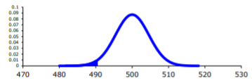.png?revision=1 "statistics of hypothesis testing")
Before calculating the probability, it is useful to see how many standard deviations away from the mean the sample mean is. Using the formula for the z-score from chapter 6, you find
\(z=\dfrac{\overline{x}-\mu_{o}}{\sigma / \sqrt{n}}=\dfrac{490-500}{25 / \sqrt{30}}=-2.19\)
This sample mean is more than two standard deviations away from the mean. That seems pretty far, but you should look at the probability too.
On TI-83/84:
\(P(\overline{x}<490 | \mu=500)=\text { normalcdf }(-1 E 99,490,500,25 \div \sqrt{30}) \approx 0.0142\)
\(P(\overline{x}<490 \mu=500)=\text { pnorm }(490,500,25 / \operatorname{sqrt}(30)) \approx 0.0142\)
There is a 1.42% chance that you could find a sample mean less than 490 when the population mean is 500 days. This is really small, so the chances are that the assumption that the population mean is 500 days is wrong, and you can reject the manufacturer’s claim. But how do you quantify really small? Is 5% or 10% or 15% really small? How do you decide?
Before you answer that question, a couple more definitions are needed.
Definition \(\PageIndex{3}\)
Test Statistic : \(z=\dfrac{\overline{x}-\mu_{o}}{\sigma / \sqrt{n}}\) since it is calculated as part of the testing of the hypothesis.
Definition \(\PageIndex{4}\)
p – value : probability that the test statistic will take on more extreme values than the observed test statistic, given that the null hypothesis is true. It is the probability that was calculated above.
Now, how small is small enough? To answer that, you really want to know the types of errors you can make.
There are actually only two errors that can be made. The first error is if you say that \(H_{o}\) is false, when in fact it is true. This means you reject \(H_{o}\) when \(H_{o}\) was true. The second error is if you say that \(H_{o}\) is true, when in fact it is false. This means you fail to reject \(H_{o}\) when \(H_{o}\) is false. The following table organizes this for you:
Type of errors:
| \(H_{o}\) true | \(H_{o}\) false | |
| Reject \(H_{o}\) | Type 1 error | No error |
| Fail to reject \(H_{o}\) | No error | Type II error |
Definition \(\PageIndex{5}\)
Type I Error is rejecting \(H_{o}\) when \(H_{o}\) is true, and
Definition \(\PageIndex{6}\)
Type II Error is failing to reject \(H_{o}\) when \(H_{o}\) is false.
Since these are the errors, then one can define the probabilities attached to each error.
Definition \(\PageIndex{7}\)
\(\alpha\) = P(type I error) = P(rejecting \(H_{o} / H_{o}\) is true)
Definition \(\PageIndex{8}\)
\(\beta\) = P(type II error) = P(failing to reject \(H_{o} / H_{o}\) is false)
\(\alpha\) is also called the level of significance .
Another common concept that is used is Power = \(1-\beta \).
Now there is a relationship between \(\alpha\) and \(\beta\). They are not complements of each other. How are they related?
If \(\alpha\) increases that means the chances of making a type I error will increase. It is more likely that a type I error will occur. It makes sense that you are less likely to make type II errors, only because you will be rejecting \(H_{o}\) more often. You will be failing to reject \(H_{o}\) less, and therefore, the chance of making a type II error will decrease. Thus, as \(\alpha\) increases, \(\beta\) will decrease, and vice versa. That makes them seem like complements, but they aren’t complements. What gives? Consider one more factor – sample size.
Consider if you have a larger sample that is representative of the population, then it makes sense that you have more accuracy then with a smaller sample. Think of it this way, which would you trust more, a sample mean of 490 if you had a sample size of 35 or sample size of 350 (assuming a representative sample)? Of course the 350 because there are more data points and so more accuracy. If you are more accurate, then there is less chance that you will make any error. By increasing the sample size of a representative sample, you decrease both \(\alpha\) and \(\beta\).
Summary of all of this:
- For a certain sample size, n , if \(\alpha\) increases, \(\beta\) decreases.
- For a certain level of significance, \(\alpha\), if n increases, \(\beta\) decreases.
Now how do you find \(\alpha\) and \(\beta\)? Well \(\alpha\) is actually chosen. There are only three values that are usually picked for \(\alpha\): 0.01, 0.05, and 0.10. \(\beta\) is very difficult to find, so usually it isn’t found. If you want to make sure it is small you take as large of a sample as you can afford provided it is a representative sample. This is one use of the Power. You want \(\beta\) to be small and the Power of the test is large. The Power word sounds good.
Which pick of \(\alpha\) do you pick? Well that depends on what you are working on. Remember in this example you are the buyer who is trying to get out of a contract to buy these batteries. If you create a type I error, you said that the batteries are bad when they aren’t, most likely the manufacturer will sue you. You want to avoid this. You might pick \(\alpha\) to be 0.01. This way you have a small chance of making a type I error. Of course this means you have more of a chance of making a type II error. No big deal right? What if the batteries are used in pacemakers and you tell the person that their pacemaker’s batteries are good for 500 days when they actually last less, that might be bad. If you make a type II error, you say that the batteries do last 500 days when they last less, then you have the possibility of killing someone. You certainly do not want to do this. In this case you might want to pick \(\alpha\) as 0.10. If both errors are equally bad, then pick \(\alpha\) as 0.05.
The above discussion is why the choice of \(\alpha\) depends on what you are researching. As the researcher, you are the one that needs to decide what \(\alpha\) level to use based on your analysis of the consequences of making each error is.
If a type I error is really bad, then pick \(\alpha\) = 0.01.
If a type II error is really bad, then pick \(\alpha\) = 0.10
If neither error is bad, or both are equally bad, then pick \(\alpha\) = 0.05
The main thing is to always pick the \(\alpha\) before you collect the data and start the test.
The above discussion was long, but it is really important information. If you don’t know what the errors of the test are about, then there really is no point in making conclusions with the tests. Make sure you understand what the two errors are and what the probabilities are for them.
Now it is time to go back to the example and put this all together. This is the basic structure of testing a hypothesis, usually called a hypothesis test. Since this one has a test statistic involving z, it is also called a z-test. And since there is only one sample, it is usually called a one-sample z-test.
Example \(\PageIndex{2}\) battery example revisited
- State the random variable and the parameter in words.
- State the null and alternative hypothesis and the level of significance.
- A random sample of size n is taken.
- The population standard derivation is known.
- The sample size is at least 30 or the population of the random variable is normally distributed.
- Find the sample statistic, test statistic, and p-value.
- Interpretation
1. x = life of battery
\(\mu\) = mean life of a XJ35 battery
2. \(H_{o} : \mu=500\) days
\(H_{A} : \mu<500\) days
\(\alpha = 0.10\) (from above discussion about consequences)
3. Every hypothesis has some assumptions that be met to make sure that the results of the hypothesis are valid. The assumptions are different for each test. This test has the following assumptions.
- This occurred in this example, since it was stated that a random sample of 30 battery lives were taken.
- This is true, since it was given in the problem.
- The sample size was 30, so this condition is met.
4. The test statistic depends on how many samples there are, what parameter you are testing, and assumptions that need to be checked. In this case, there is one sample and you are testing the mean. The assumptions were checked above.
Sample statistic:
\(\overline{x} = 490\)
Test statistic:
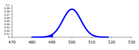.png?revision=1 "statistics of hypothesis testing")
Using TI-83/84:
\(P(\overline{x}<490 | \mu=500)=\text { normalcdf }(-1 \mathrm{E} 99,490,500,25 / \sqrt{30}) \approx 0.0142\)
\(P(\overline{x}<490 | \mu=500)=\operatorname{pnorm}(490,500,25 / \operatorname{sqrt}(30)) \approx 0.0142\)
5. Now what? Well, this p-value is 0.0142. This is a lot smaller than the amount of error you would accept in the problem -\(\alpha\) = 0.10. That means that finding a sample mean less than 490 days is unusual to happen if \(H_{o}\) is true. This should make you think that \(H_{o}\) is not true. You should reject \(H_{o}\).
In fact, in general:
Reject \(H_{o}\) if the p-value < \(\alpha\) and
Fail to reject \(H_{o}\) if the p-value \(\geq \alpha\).
6. Since you rejected \(H_{o}\), what does this mean in the real world? That is what goes in the interpretation. Since you rejected the claim by the manufacturer that the mean life of the batteries is 500 days, then you now can believe that your hypothesis was correct. In other words, there is enough evidence to show that the mean life of the battery is less than 500 days.
Now that you know that the batteries last less than 500 days, should you cancel the contract? Statistically, there is evidence that the batteries do not last as long as the manufacturer says they should. However, based on this sample there are only ten days less on average that the batteries last. There may not be practical significance in this case. Ten days do not seem like a large difference. In reality, if the batteries are used in pacemakers, then you would probably tell the patient to have the batteries replaced every year. You have a large buffer whether the batteries last 490 days or 500 days. It seems that it might not be worth it to break the contract over ten days. What if the 10 days was practically significant? Are there any other things you should consider? You might look at the business relationship with the manufacturer. You might also look at how much it would cost to find a new manufacturer. These are also questions to consider before making any changes. What this discussion should show you is that just because a hypothesis has statistical significance does not mean it has practical significance. The hypothesis test is just one part of a research process. There are other pieces that you need to consider.
That’s it. That is what a hypothesis test looks like. All hypothesis tests are done with the same six steps. Those general six steps are outlined below.
- State the random variable and the parameter in words. This is where you are defining what the unknowns are in this problem. x = random variable \(\mu\) = mean of random variable, if the parameter of interest is the mean. There are other parameters you can test, and you would use the appropriate symbol for that parameter.
- State the null and alternative hypotheses and the level of significance \(H_{o} : \mu=\mu_{o}\), where \(\mu_{o}\) is the known mean \(H_{A} : \mu<\mu_{o}\) \(H_{A} : \mu>\mu_{o}\), use the appropriate one for your problem \(H_{A} : \mu \neq \mu_{o}\) Also, state your \(\alpha\) level here.
- State and check the assumptions for a hypothesis test. Each hypothesis test has its own assumptions. They will be stated when the different hypothesis tests are discussed.
- Find the sample statistic, test statistic, and p-value. This depends on what parameter you are working with, how many samples, and the assumptions of the test. The p-value depends on your \(H_{A}\). If you are doing the \(H_{A}\) with the less than, then it is a left-tailed test, and you find the probability of being in that left tail. If you are doing the \(H_{A}\) with the greater than, then it is a right-tailed test, and you find the probability of being in the right tail. If you are doing the \(H_{A}\) with the not equal to, then you are doing a two-tail test, and you find the probability of being in both tails. Because of symmetry, you could find the probability in one tail and double this value to find the probability in both tails.
- Conclusion This is where you write reject \(H_{o}\) or fail to reject \(H_{o}\). The rule is: if the p-value < \(\alpha\), then reject \(H_{o}\). If the p-value \(\geq \alpha\), then fail to reject \(H_{o}\).
- Interpretation This is where you interpret in real world terms the conclusion to the test. The conclusion for a hypothesis test is that you either have enough evidence to show \(H_{A}\) is true, or you do not have enough evidence to show \(H_{A}\) is true.
Sorry, one more concept about the conclusion and interpretation. First, the conclusion is that you reject \(H_{o}\) or you fail to reject \(H_{o}\). Why was it said like this? It is because you never accept the null hypothesis. If you wanted to accept the null hypothesis, then why do the test in the first place? In the interpretation, you either have enough evidence to show \(H_{A}\) is true, or you do not have enough evidence to show \(H_{A}\) is true. You wouldn’t want to go to all this work and then find out you wanted to accept the claim. Why go through the trouble? You always want to show that the alternative hypothesis is true. Sometimes you can do that and sometimes you can’t. It doesn’t mean you proved the null hypothesis; it just means you can’t prove the alternative hypothesis. Here is an example to demonstrate this.
Example \(\PageIndex{3}\) conclusion in hypothesis tests
In the U.S. court system a jury trial could be set up as a hypothesis test. To really help you see how this works, let’s use OJ Simpson as an example. In the court system, a person is presumed innocent until he/she is proven guilty, and this is your null hypothesis. OJ Simpson was a football player in the 1970s. In 1994 his ex-wife and her friend were killed. OJ Simpson was accused of the crime, and in 1995 the case was tried. The prosecutors wanted to prove OJ was guilty of killing his wife and her friend, and that is the alternative hypothesis
\(H_{0}\): OJ is innocent of killing his wife and her friend
\(H_{A}\): OJ is guilty of killing his wife and her friend
In this case, a verdict of not guilty was given. That does not mean that he is innocent of this crime. It means there was not enough evidence to prove he was guilty. Many people believe that OJ was guilty of this crime, but the jury did not feel that the evidence presented was enough to show there was guilt. The verdict in a jury trial is always guilty or not guilty!
The same is true in a hypothesis test. There is either enough or not enough evidence to show that alternative hypothesis. It is not that you proved the null hypothesis true.
When identifying hypothesis, it is important to state your random variable and the appropriate parameter you want to make a decision about. If count something, then the random variable is the number of whatever you counted. The parameter is the proportion of what you counted. If the random variable is something you measured, then the parameter is the mean of what you measured. (Note: there are other parameters you can calculate, and some analysis of those will be presented in later chapters.)
Example \(\PageIndex{4}\) stating hypotheses
Identify the hypotheses necessary to test the following statements:
- The average salary of a teacher is more than $30,000.
- The proportion of students who like math is less than 10%.
- The average age of students in this class differs from 21.
a. x = salary of teacher
\(\mu\) = mean salary of teacher
The guess is that \(\mu>\$ 30,000\) and that is the alternative hypothesis.
The null hypothesis has the same parameter and number with an equal sign.
\(\begin{array}{l}{H_{0} : \mu=\$ 30,000} \\ {H_{A} : \mu>\$ 30,000}\end{array}\)
b. x = number od students who like math
p = proportion of students who like math
The guess is that p < 0.10 and that is the alternative hypothesis.
\(\begin{array}{l}{H_{0} : p=0.10} \\ {H_{A} : p<0.10}\end{array}\)
c. x = age of students in this class
\(\mu\) = mean age of students in this class
The guess is that \(\mu \neq 21\) and that is the alternative hypothesis.
\(\begin{array}{c}{H_{0} : \mu=21} \\ {H_{A} : \mu \neq 21}\end{array}\)
Example \(\PageIndex{5}\) Stating Type I and II Errors and Picking Level of Significance
- The plant-breeding department at a major university developed a new hybrid raspberry plant called YumYum Berry. Based on research data, the claim is made that from the time shoots are planted 90 days on average are required to obtain the first berry with a standard deviation of 9.2 days. A corporation that is interested in marketing the product tests 60 shoots by planting them and recording the number of days before each plant produces its first berry. The sample mean is 92.3 days. The corporation wants to know if the mean number of days is more than the 90 days claimed. State the type I and type II errors in terms of this problem, consequences of each error, and state which level of significance to use.
- A concern was raised in Australia that the percentage of deaths of Aboriginal prisoners was higher than the percent of deaths of non-indigenous prisoners, which is 0.27%. State the type I and type II errors in terms of this problem, consequences of each error, and state which level of significance to use.
a. x = time to first berry for YumYum Berry plant
\(\mu\) = mean time to first berry for YumYum Berry plant
\(\begin{array}{l}{H_{0} : \mu=90} \\ {H_{A} : \mu>90}\end{array}\)
Type I Error: If the corporation does a type I error, then they will say that the plants take longer to produce than 90 days when they don’t. They probably will not want to market the plants if they think they will take longer. They will not market them even though in reality the plants do produce in 90 days. They may have loss of future earnings, but that is all.
Type II error: The corporation do not say that the plants take longer then 90 days to produce when they do take longer. Most likely they will market the plants. The plants will take longer, and so customers might get upset and then the company would get a bad reputation. This would be really bad for the company.
Level of significance: It appears that the corporation would not want to make a type II error. Pick a 10% level of significance, \(\alpha = 0.10\).
b. x = number of Aboriginal prisoners who have died
p = proportion of Aboriginal prisoners who have died
\(\begin{array}{l}{H_{o} : p=0.27 \%} \\ {H_{A} : p>0.27 \%}\end{array}\)
Type I error: Rejecting that the proportion of Aboriginal prisoners who died was 0.27%, when in fact it was 0.27%. This would mean you would say there is a problem when there isn’t one. You could anger the Aboriginal community, and spend time and energy researching something that isn’t a problem.
Type II error: Failing to reject that the proportion of Aboriginal prisoners who died was 0.27%, when in fact it is higher than 0.27%. This would mean that you wouldn’t think there was a problem with Aboriginal prisoners dying when there really is a problem. You risk causing deaths when there could be a way to avoid them.
Level of significance: It appears that both errors may be issues in this case. You wouldn’t want to anger the Aboriginal community when there isn’t an issue, and you wouldn’t want people to die when there may be a way to stop it. It may be best to pick a 5% level of significance, \(\alpha = 0.05\).
Hypothesis testing is really easy if you follow the same recipe every time. The only differences in the various problems are the assumptions of the test and the test statistic you calculate so you can find the p-value. Do the same steps, in the same order, with the same words, every time and these problems become very easy.
Exercise \(\PageIndex{1}\)
For the problems in this section, a question is being asked. This is to help you understand what the hypotheses are. You are not to run any hypothesis tests and come up with any conclusions in this section.
- Eyeglassomatic manufactures eyeglasses for different retailers. They test to see how many defective lenses they made in a given time period and found that 11% of all lenses had defects of some type. Looking at the type of defects, they found in a three-month time period that out of 34,641 defective lenses, 5865 were due to scratches. Are there more defects from scratches than from all other causes? State the random variable, population parameter, and hypotheses.
- According to the February 2008 Federal Trade Commission report on consumer fraud and identity theft, 23% of all complaints in 2007 were for identity theft. In that year, Alaska had 321 complaints of identity theft out of 1,432 consumer complaints ("Consumer fraud and," 2008). Does this data provide enough evidence to show that Alaska had a lower proportion of identity theft than 23%? State the random variable, population parameter, and hypotheses.
- The Kyoto Protocol was signed in 1997, and required countries to start reducing their carbon emissions. The protocol became enforceable in February 2005. In 2004, the mean CO2 emission was 4.87 metric tons per capita. Is there enough evidence to show that the mean CO2 emission is lower in 2010 than in 2004? State the random variable, population parameter, and hypotheses.
- The FDA regulates that fish that is consumed is allowed to contain 1.0 mg/kg of mercury. In Florida, bass fish were collected in 53 different lakes to measure the amount of mercury in the fish. The data for the average amount of mercury in each lake is in Example \(\PageIndex{5}\) ("Multi-disciplinary niser activity," 2013). Do the data provide enough evidence to show that the fish in Florida lakes has more mercury than the allowable amount? State the random variable, population parameter, and hypotheses.
- Eyeglassomatic manufactures eyeglasses for different retailers. They test to see how many defective lenses they made in a given time period and found that 11% of all lenses had defects of some type. Looking at the type of defects, they found in a three-month time period that out of 34,641 defective lenses, 5865 were due to scratches. Are there more defects from scratches than from all other causes? State the type I and type II errors in this case, consequences of each error type for this situation from the perspective of the manufacturer, and the appropriate alpha level to use. State why you picked this alpha level.
- According to the February 2008 Federal Trade Commission report on consumer fraud and identity theft, 23% of all complaints in 2007 were for identity theft. In that year, Alaska had 321 complaints of identity theft out of 1,432 consumer complaints ("Consumer fraud and," 2008). Does this data provide enough evidence to show that Alaska had a lower proportion of identity theft than 23%? State the type I and type II errors in this case, consequences of each error type for this situation from the perspective of the state of Arizona, and the appropriate alpha level to use. State why you picked this alpha level.
- The Kyoto Protocol was signed in 1997, and required countries to start reducing their carbon emissions. The protocol became enforceable in February 2005. In 2004, the mean CO2 emission was 4.87 metric tons per capita. Is there enough evidence to show that the mean CO2 emission is lower in 2010 than in 2004? State the type I and type II errors in this case, consequences of each error type for this situation from the perspective of the agency overseeing the protocol, and the appropriate alpha level to use. State why you picked this alpha level.
- The FDA regulates that fish that is consumed is allowed to contain 1.0 mg/kg of mercury. In Florida, bass fish were collected in 53 different lakes to measure the amount of mercury in the fish. The data for the average amount of mercury in each lake is in Example \(\PageIndex{5}\) ("Multi-disciplinary niser activity," 2013). Do the data provide enough evidence to show that the fish in Florida lakes has more mercury than the allowable amount? State the type I and type II errors in this case, consequences of each error type for this situation from the perspective of the FDA, and the appropriate alpha level to use. State why you picked this alpha level.
1. \(H_{o} : p=0.11, H_{A} : p>0.11\)
3. \(H_{o} : \mu=4.87 \text { metric tons per capita, } H_{A} : \mu<4.87 \text { metric tons per capita }\)
5. See solutions
7. See solutions
Help | Advanced Search
Mathematics > Statistics Theory
Title: federated nonparametric hypothesis testing with differential privacy constraints: optimal rates and adaptive tests.
Abstract: Federated learning has attracted significant recent attention due to its applicability across a wide range of settings where data is collected and analyzed across disparate locations. In this paper, we study federated nonparametric goodness-of-fit testing in the white-noise-with-drift model under distributed differential privacy (DP) constraints. We first establish matching lower and upper bounds, up to a logarithmic factor, on the minimax separation rate. This optimal rate serves as a benchmark for the difficulty of the testing problem, factoring in model characteristics such as the number of observations, noise level, and regularity of the signal class, along with the strictness of the $(\epsilon,\delta)$-DP requirement. The results demonstrate interesting and novel phase transition phenomena. Furthermore, the results reveal an interesting phenomenon that distributed one-shot protocols with access to shared randomness outperform those without access to shared randomness. We also construct a data-driven testing procedure that possesses the ability to adapt to an unknown regularity parameter over a large collection of function classes with minimal additional cost, all while maintaining adherence to the same set of DP constraints.
| Comments: | 77 pages total; consisting of a main article (28 pages) and supplement (49 pages) |
| Subjects: | Statistics Theory (math.ST); Machine Learning (cs.LG); Machine Learning (stat.ML) |
| classes: | 62G10, 62C20, 68P27, 62F30 |
| Cite as: | [math.ST] |
| (or [math.ST] for this version) | |
| Focus to learn more arXiv-issued DOI via DataCite |
Submission history
Access paper:.
- HTML (experimental)
- Other Formats
References & Citations
- Google Scholar
- Semantic Scholar
BibTeX formatted citation
Bibliographic and Citation Tools
Code, data and media associated with this article, recommenders and search tools.
- Institution
arXivLabs: experimental projects with community collaborators
arXivLabs is a framework that allows collaborators to develop and share new arXiv features directly on our website.
Both individuals and organizations that work with arXivLabs have embraced and accepted our values of openness, community, excellence, and user data privacy. arXiv is committed to these values and only works with partners that adhere to them.
Have an idea for a project that will add value for arXiv's community? Learn more about arXivLabs .
IMAGES
VIDEO
COMMENTS
Hypothesis Testing | A Step-by-Step Guide with Easy Examples. Published on November 8, 2019 by Rebecca Bevans.Revised on June 22, 2023. Hypothesis testing is a formal procedure for investigating our ideas about the world using statistics.It is most often used by scientists to test specific predictions, called hypotheses, that arise from theories.
A hypothesis test is a formal procedure to check if a hypothesis is true or not. Examples of claims that can be checked: The average height of people in Denmark is more than 170 cm. The share of left handed people in Australia is not 10%. The average income of dentists is less the average income of lawyers.
Hypothesis testing is a form of inferential statistics that allows us to draw conclusions about an entire population based on a representative sample. You gain tremendous benefits by working with a sample. In most cases, it is simply impossible to observe the entire population to understand its properties.
The above image shows a table with some of the most common test statistics and their corresponding tests or models.. A statistical hypothesis test is a method of statistical inference used to decide whether the data sufficiently support a particular hypothesis. A statistical hypothesis test typically involves a calculation of a test statistic.Then a decision is made, either by comparing the ...
A hypothesis test consists of five steps: 1. State the hypotheses. State the null and alternative hypotheses. These two hypotheses need to be mutually exclusive, so if one is true then the other must be false. 2. Determine a significance level to use for the hypothesis. Decide on a significance level.
In hypothesis testing, the goal is to see if there is sufficient statistical evidence to reject a presumed null hypothesis in favor of a conjectured alternative hypothesis.The null hypothesis is usually denoted \(H_0\) while the alternative hypothesis is usually denoted \(H_1\). An hypothesis test is a statistical decision; the conclusion will either be to reject the null hypothesis in favor ...
Hypothesis testing involves five key steps, each critical to validating a research hypothesis using statistical methods: Formulate the Hypotheses: Write your research hypotheses as a null hypothesis (H 0) and an alternative hypothesis (H A ). Data Collection: Gather data specifically aimed at testing the hypothesis.
Unit 12: Significance tests (hypothesis testing) Significance tests give us a formal process for using sample data to evaluate the likelihood of some claim about a population value. Learn how to conduct significance tests and calculate p-values to see how likely a sample result is to occur by random chance. You'll also see how we use p-values ...
This is also the case with hypothesis testing: even if we fail to reject the null hypothesis, we typically do not accept the null hypothesis as true. Failing to find strong evidence for the alternative hypothesis is not equivalent to accepting the null hypothesis. 17 H 0: The average cost is $650 per month, μ = $650.
S.3 Hypothesis Testing. In reviewing hypothesis tests, we start first with the general idea. Then, we keep returning to the basic procedures of hypothesis testing, each time adding a little more detail. The general idea of hypothesis testing involves: Making an initial assumption. Collecting evidence (data).
Step 7: Based on steps 5 and 6, draw a conclusion about H0. If the F\calculated from the data is larger than the Fα, then you are in the rejection region and you can reject the null hypothesis with (1 − α) level of confidence. Note that modern statistical software condenses steps 6 and 7 by providing a p -value.
8.1 Inferential Statistics and Hypothesis Testing 8.2 Four Steps to Hypothesis Testing 8.3 Hypothesis Testing and Sampling Distributions 8.4 Making a Decision: 8.5 Testing a Research Using the z Test 8.6 Research in Focus: Directional Versus Nondirectional Tests 8.7 Measuring the Size of an Effect: Cohen's d 8.8 Effect Size, Power, and
Hypothesis testing is a formal procedure for investigating our ideas about the world. It allows you to statistically test your predictions. ... Test statistics | Definition, Interpretation, and Examples The test statistic is a number, calculated from a statistical test, used to find if your data could have occurred under the null hypothesis. 254.
Photo from StepUp Analytics. Hypothesis testing is a method of statistical inference that considers the null hypothesis H₀ vs. the alternative hypothesis Ha, where we are typically looking to assess evidence against H₀. Such a test is used to compare data sets against one another, or compare a data set against some external standard. The former being a two sample test (independent or ...
The test statistic is a number calculated from a statistical test of a hypothesis. It shows how closely your observed data match the distribution expected under the null hypothesis of that statistical test. The test statistic is used to calculate the p value of your results, helping to decide whether to reject your null hypothesis.
Hypothesis testing is a statistical method used to determine if there is enough evidence in a sample data to draw conclusions about a population. It involves formulating two competing hypotheses, the null hypothesis (H0) and the alternative hypothesis (Ha), and then collecting data to assess the evidence.
What is Hypothesis Testing? Hypothesis testing in statistics is a tool that is used to make inferences about the population data. It is also used to check if the results of an experiment are valid. What is the z Test in Hypothesis Testing? The z test in hypothesis testing is used to find the z test statistic for normally distributed data. The z ...
This tests whether the population parameter is equal to, versus less than, some specific value. Ho: μ = 12 vs. H1: μ < 12. The critical region is in the left tail and the critical value is a negative value that defines the rejection zone. Figure 3.1.3 3.1. 3: The rejection zone for a left-sided hypothesis test.
HYPOTHESIS TESTING. A clinical trial begins with an assumption or belief, and then proceeds to either prove or disprove this assumption. In statistical terms, this belief or assumption is known as a hypothesis. Counterintuitively, what the researcher believes in (or is trying to prove) is called the "alternate" hypothesis, and the opposite ...
Introduction to Hypotheses Tests. Hypothesis testing is a statistical tool used to make decisions based on data. It involves making assumptions about a population parameter and testing its validity using a population sample. Hypothesis tests help us draw conclusions and make informed decisions in various fields like business, research, and science.
Statistics: Hypothesis Testing . A hypothesis is a claim made about a population. A hypothesis test uses sample data to test the validity of the claim. This handout will define the basic elements of hypothesis testing and provide the steps to perform hypothesis tests using the P-value method and the critical value
The hypothesis testing is a statistical method that allows to formulate and evaluate an hypothesis about the population based on sample data. So, it is a form of inferential statistics. This process starts with a hypothesis of the population parameters, also called null hypothesis, that needs to be tested, while the alternative hypothesis (H1 ...
Unit 14: Prepare for the 2022 AP®︎ Statistics Exam. Mastery unavailable. Prepare for the exam. Up next for you: Course challenge Test your knowledge of the skills in this course. Start Course challenge.
Bibliography. A scientific hypothesis is a tentative, testable explanation for a phenomenon in the natural world. It's the initial building block in the scientific method. Many describe it as an ...
Hypothesis Testing Step 1: State the Hypotheses. In all three examples, our aim is to decide between two opposing points of view, Claim 1 and Claim 2. In hypothesis testing, Claim 1 is called the null hypothesis (denoted " Ho "), and Claim 2 plays the role of the alternative hypothesis (denoted " Ha ").
DATAtab is a modern statistics software, with unique user-friendliness. Statistical analyses are done with just a few clicks, so DATAtab is perfect for statistics beginners and for professionals who want more flow in the user experience. ... Here you will find everything about hypothesis testing: One sample t-test, Unpaired t-test, Paired t ...
Hypothesis Testing • … "one of the most important tools for the application of statistics to business problems" • We are interested in making claims about a population from a sample of data • Those claims are usually stated as hypotheses and we use hypothesis testing to determine if a claim (hypothesis) is supported or not with statistical evidence EC255: Chapter 9 5
Test Statistic: z = x¯¯¯ −μo σ/ n−−√ z = x ¯ − μ o σ / n since it is calculated as part of the testing of the hypothesis. Definition 7.1.4 7.1. 4. p - value: probability that the test statistic will take on more extreme values than the observed test statistic, given that the null hypothesis is true.
Federated learning has attracted significant recent attention due to its applicability across a wide range of settings where data is collected and analyzed across disparate locations. In this paper, we study federated nonparametric goodness-of-fit testing in the white-noise-with-drift model under distributed differential privacy (DP) constraints. We first establish matching lower and upper ...