problem solving on velocity

Exam Center
Ticket Center
Flash Cards
Straight Line Motion

Solved Speed, Velocity, and Acceleration Problems

Simple problems on speed, velocity, and acceleration with descriptive answers are presented for the AP Physics 1 exam and college students. In each solution, you can find a brief tutorial.

Speed and velocity Problems:

Problem (1): What is the speed of a rocket that travels $8000\,{\rm m}$ in $13\,{\rm s}$?

Solution : Speed is defined in physics as the total distance divided by the elapsed time, so the rocket's speed is \[\text{speed}=\frac{8000}{13}=615.38\,{\rm m/s}\]

Problem (2): How long will it take if you travel $400\,{\rm km}$ with an average speed of $100\,{\rm m/s}$?

Solution : Average speed is the ratio of the total distance to the total time. Thus, the elapsed time is \begin{align*} t&=\frac{\text{total distance}}{\text{average speed}}\\ \\ &=\frac{400\times 10^{3}\,{\rm m}}{100\,{\rm m/s}}\\ \\ &=4000\,{\rm s}\end{align*} To convert it to hours, it must be divided by $3600\,{\rm s}$ which gives $t=1.11\,{\rm h}$.

Problem (3): A person walks $100\,{\rm m}$ in $5$ minutes, then $200\,{\rm m}$ in $7$ minutes, and finally $50\,{\rm m}$ in $4$ minutes. Find its average speed.

Solution : First find its total distance traveled ($D$) by summing all distances in each section, which gets $D=100+200+50=350\,{\rm m}$. Now, by definition of average speed, divide it by the total time elapsed $T=5+7+4=16$ minutes.

But keep in mind that since the distance is in SI units, so the time traveled must also be in SI units, which is $\rm s$. Therefore, we have\begin{align*}\text{average speed}&=\frac{\text{total distance} }{\text{total time} }\\ \\ &=\frac{350\,{\rm m}}{16\times 60\,{\rm s}}\\ \\&=0.36\,{\rm m/s}\end{align*}

Problem (4): A person walks $750\,{\rm m}$ due north, then $250\,{\rm m}$ due east. If the entire walk takes $12$ minutes, find the person's average velocity.

Solution : Average velocity , $\bar{v}=\frac{\Delta x}{\Delta t}$, is displacement divided by the elapsed time. Displacement is also a vector that obeys the addition vector rules. Thus, in this velocity problem, add each displacement to get the total displacement .

In the first part, displacement is $\Delta x_1=750\,\hat{j}$ (due north) and in the second part $\Delta x_2=250\,\hat{i}$ (due east). The total displacement vector is $\Delta x=\Delta x_1+\Delta x_2=750\,\hat{i}+250\,\hat{j}$ with magnitude of \begin{align*}|\Delta x|&=\sqrt{(750)^{2}+(250)^{2}}\\ \\&=790.5\,{\rm m}\end{align*} In addition, the total elapsed time is $t=12\times 60$ seconds. Therefore, the magnitude of the average velocity is \[\bar{v}=\frac{790.5}{12\times 60}=1.09\,{\rm m/s}\]

Problem (5): An object moves along a straight line. First, it travels at a velocity of $12\,{\rm m/s}$ for $5\,{\rm s}$ and then continues in the same direction with $20\,{\rm m/s}$ for $3\,{\rm s}$. What is its average speed?

Solution: Average velocity is displacement divided by elapsed time, i.e., $\bar{v}\equiv \frac{\Delta x_{tot}}{\Delta t_{tot}}$.

Here, the object goes through two stages with two different displacements, so add them to find the total displacement. Thus,\[\bar{v}=\frac{x_1 + x_2}{t_1 +t_2}\] Again, to find the displacement, we use the same equation as the average velocity formula, i.e., $x=vt$. Thus, displacements are obtained as $x_1=v_1\,t_1=12\times 5=60\,{\rm m}$ and $x_2=v_2\,t_2=20\times 3=60\,{\rm m}$. Therefore, we have \begin{align*} \bar{v}&=\frac{x_1+x_2}{t_1+t_2}\\ \\&=\frac{60+60}{5+3}\\ \\&=\boxed{15\,{\rm m/s}}\end{align*}

Problem (6): A plane flies the distance between two cities in $1$ hour and $30$ minutes with a velocity of $900\,{\rm km/h}$. Another plane covers that distance at $600\,{\rm km/h}$. What is the flight time of the second plane?

Solution: first find the distance between two cities using the average velocity formula $\bar{v}=\frac{\Delta x}{\Delta t}$ as below \begin{align*} x&=vt\\&=900\times 1.5\\&=1350\,{\rm km}\end{align*} where we wrote one hour and a half minutes as $1.5\,\rm h$. Now use again the same kinematic equation above to find the time required for another plane \begin{align*} t&=\frac xv\\ \\ &=\frac{1350\,\rm km}{600\,\rm km/h}\\ \\&=2.25\,{\rm h}\end{align*} Thus, the time for the second plane is $2$ hours and $0.25$ of an hour, which converts to minutes as $2$ hours and ($0.25\times 60=15$) minutes.

Problem (7): To reach a park located south of his jogging path, Henry runs along a 15-kilometer route. If he completes the journey in 1.5 hours, determine his speed and velocity.

Solution: Henry travels his route to the park without changing direction along a straight line. Therefore, the total distance traveled in one direction equals the displacement, i.e, \[\text{distance traveled}=\Delta x=15\,\rm km\]Velocity is displacement divided by the time of travel \begin{align*} \text{velocity}&=\frac{\text{displacement}}{\text{time of travel}} \\\\ &=\frac{15\,\rm km}{1.5\,\rm h} \\\\ &=\boxed{10\,\rm km/h}\end{align*} and by definition, its average speed is \begin{align*} \text{speed}&=\frac{\text{distance covered}}{\text{time interval}}\\\\&=\frac{15\,\rm km}{1.5\,\rm h}\\\\&=\boxed{10\,\rm km/h}\end{align*} Thus, Henry's velocity is $10\,\rm km/h$ to the south, and its speed is $10\,\rm km/h$. As you can see, speed is simply a positive number, with units but velocity specifies the direction in which the object is moving.

Problem (8): In 15 seconds, a football player covers the distance from his team's goal line to the opposing team's goal line and back to the midway point of the field having 100-yard-length. Find, (a) his average speed, and (b) the magnitude of the average velocity.

Solution: The total length of the football field is $100$ yards or in meters, $L=91.44\,\rm m$. Going from one goal's line to the other and back to the midpoint of the field takes $15\,\rm s$ and covers a distance of $D=100+50=150\,\rm yd$.

average speed and velocity at football field

Distance divided by the time of travel gets the average speed, \[\text{speed}=\frac{150\times 0.91}{15}=9.1\,\rm m/s\] To find the average velocity, we must find the displacement of the player between the initial and final points.

The initial point is her own goal line and her final position is the midpoint of the field, so she has displaced a distance of $\Delta x=50\,\rm yd$ or $\Delta x=50\times 0.91=45.5\,\rm m$. Therefore, her velocity is calculated as follows \begin{align*} \text{velocity}&=\frac{\text{displacement}}{\text{time elapsed}} \\\\ &=\frac{45.5\,\rm m}{15\,\rm s} \\\\&=\boxed{3.03\quad \rm m/s}\end{align*} Contrary to the previous problem, here the motion is not in one direction, hence, the displacement is not equal to the distance traveled. Accordingly, the average speed is not equal to the magnitude of the average velocity.

Problem (9): You begin at a pillar and run towards the east (the positive $x$ direction) for $250\,\rm m$ at an average speed of $5\,\rm m/s$. After that, you run towards the west for $300\,\rm m$ at an average speed of $4\,\rm m/s$ until you reach a post. Calculate (a) your average speed from pillar to post, and (b) your average velocity from pillar to post.

Solution : First, you traveled a distance of $L_1=250\,\rm m$ toward east (or $+x$ direction) at $5\,\rm m/s$. Time of travel in this route is obtained as follows \begin{align*} t_1&=\frac{L_1}{v_1}\\\\ &=\frac{250}{5}\\\\&=50\,\rm s\end{align*} Likewise, traveling a distance of $L_2=300\,\rm m$ at $v_2=4\,\rm m/s$ takes \[t_2=\frac{300}{4}=75\,\rm s\] (a) Average speed is defined as the distance traveled (or path length) divided by the total time of travel \begin{align*} v&=\frac{\text{path length}}{\text{time of travel}} \\\\ &=\frac{L_1+L_2}{t_1+t_2}\\\\&=\frac{250+300}{50+75} \\\\&=4.4\,\rm m/s\end{align*} Therefore, you travel between these two pillars in $125\,\rm s$ and with an average speed of $4.4\,\rm m/s$.

(b) Average velocity requires finding the displacement between those two points. In the first case, you move $250\,\rm m$ toward $+x$ direction, i.e., $L_1=+250\,\rm m$. Similarly, on the way back, you move $300\,\rm m$ toward the west ($-x$ direction) or $L_2=-300\,\rm m$. Adding these two gives us the total displacement between the initial point and the final point, \begin{align*} L&=L_1+L_2 \\\\&=(+250)+(-300) \\\\ &=-50\,\rm m\end{align*} The minus sign indicates that you are generally displaced toward the west.

Finally, the average velocity is obtained as follows: \begin{align*} \text{average velocity}&=\frac{\text{displacement}}{\text{time of travel}} \\\\ &=\frac{-50}{125} \\\\&=-0.4\,\rm m/s\end{align*} A negative average velocity indicating motion to the left along the $x$-axis.

This speed problem better makes it clear to us the difference between average speed and average speed. Unlike average speed, which is always a positive number, the average velocity in a straight line can be either positive or negative.

Problem (10): What is the average speed for the round trip of a car moving uphill at 40 km/h and then back downhill at 60 km/h?

Solution : Assuming the length of the hill to be $L$, the total distance traveled during this round trip is $2L$ since $L_{up}=L_{down}=L$. However, the time taken for going uphill and downhill was not provided. We can write them in terms of the hill's length $L$ as $t=\frac L v$.

Applying the definition of average speed gives us \begin{align*} v&=\frac{\text{distance traveled}}{\text{total time}} \\\\ &=\frac{L_{up}+L_{down}}{t_{up}+t_{down}} \\\\ &=\cfrac{2L}{\cfrac{L}{v_{up}}+\cfrac{L}{v_{down}}} \end{align*} By reorganizing this expression, we obtain a formula that is useful for solving similar problems in the AP Physics 1 exams. \[\text{average speed}=\frac{2v_{up} \times v_{down}}{v_{up}+v_{down}}\] Substituting the numerical values into this, yields \begin{align*} v&=\frac{2(40\times 60)}{40+60} \\\\ &=\boxed{48\,\rm m/s}\end{align*} What if we were asked for the average velocity instead? During this round trip, the car returns to its original position, and thus its displacement, which defines the average velocity, is zero. Therefore, \[\text{average velocity}=0\,\rm m/s\]

Acceleration Problems

Problem (9): A car moves from rest to a speed of $45\,\rm m/s$ in a time interval of $15\,\rm s$. At what rate does the car accelerate?

Solution : The car is initially at rest, $v_1=0$, and finally reaches $v_2=45\,\rm m/s$ in a time interval $\Delta t=15\,\rm s$. Average acceleration is the change in velocity, $\Delta v=v_2-v_1$, divided by the elapsed time $\Delta t$, so \[\bar{a}=\frac{45-0}{15}=\boxed{3\,\rm m/s^2} \]

Problem (10): A car moving at a velocity of $15\,{\rm m/s}$, uniformly slows down. It comes to a complete stop in $10\,{\rm s}$. What is its acceleration?

Solution: Let the car's uniform velocity be $v_1$ and its final velocity $v_2=0$. Average acceleration is the difference in velocities divided by the time taken, so we have: \begin{align*}\bar{a}&=\frac{\Delta v}{\Delta t}\\\\&=\frac{v_2-v_1}{\Delta t}\\\\&=\frac{0-15}{10}\\\\ &=\boxed{-1.5\,{\rm m/s^2}}\end{align*}The minus sign indicates the direction of the acceleration vector, which is toward the $-x$ direction.

Problem (11): A car moves from rest to a speed of $72\,{\rm km/h}$ in $4\,{\rm s}$. Find the acceleration of the car.

Solution: Known: $v_1=0$, $v_2=72\,{\rm km/h}$, $\Delta t=4\,{\rm s}$. Average acceleration is defined as the difference in velocities divided by the time interval between those points \begin{align*}\bar{a}&=\frac{v_2-v_1}{t_2-t_1}\\\\&=\frac{20-0}{4}\\\\&=5\,{\rm m/s^2}\end{align*} In above, we converted $\rm km/h$ to the SI unit of velocity ($\rm m/s$) as \[1\,\frac{km}{h}=\frac {1000\,m}{3600\,s}=\frac{10}{36}\, \rm m/s\] so we get \[72\,\rm km/h=72\times \frac{10}{36}=20\,\rm m/s\]

Problem (12): A race car accelerates from an initial velocity of $v_i=10\,{\rm m/s}$ to a final velocity of $v_f = 30\,{\rm m/s}$ in a time interval of $2\,{\rm s}$. Determine its average acceleration.

Solution: A change in the velocity of an object $\Delta v$ over a time interval $\Delta t$ is defined as an average acceleration. Known: $v_i=10\,{\rm m/s}$, $v_f = 30\,{\rm m/s}$, $\Delta t=2\,{\rm s}$. Applying definition of average acceleration, we get \begin{align*}\bar{a}&=\frac{v_f-v_i}{\Delta t}\\&=\frac{30-10}{2}\\&=10\,{\rm m/s^2}\end{align*}

Problem (13): A motorcycle starts its trip along a straight line with a velocity of $10\,{\rm m/s}$ and ends with $20\,{\rm m/s}$ in the opposite direction in a time interval of $2\,{\rm s}$. What is the average acceleration of the car?

Solution: Known: $v_i=10\,{\rm m/s}$, $v_f=-20\,{\rm m/s}$, $\Delta t=2\,{\rm s}$, $\bar{a}=?$. Using average acceleration definition we have \begin{align*}\bar{a}&=\frac{v_f-v_i}{\Delta t}\\\\&=\frac{(-20)-10}{2}\\\\ &=\boxed{-15\,{\rm m/s^2}}\end{align*}Recall that in the definition above, velocities are vector quantities. The final velocity is in the opposite direction from the initial velocity so a negative must be included.

Problem (14): A ball is thrown vertically up into the air by a boy. After $4$ seconds, it reaches the highest point of its path. How fast does the ball leave the boy's hand?

Solution : At the highest point, the ball has zero speed, $v_2=0$. It takes the ball $4\,\rm s$ to reach that point. In this problem, our unknown is the initial speed of the ball, $v_1=?$. Here, the ball accelerates at a constant rate of $g=-9.8\,\rm m/s^2$ in the presence of gravity.

When the ball is tossed upward, the only external force that acts on it is the gravity force.

Using the average acceleration formula $\bar{a}=\frac{\Delta v}{\Delta t}$ and substituting the numerical values into this, we will have \begin{gather*} \bar{a}=\frac{\Delta v}{\Delta t} \\\\ -9.8=\frac{0-v_1}{4} \\\\ \Rightarrow \boxed{v_1=39.2\,\rm m/s} \end{gather*} Note that $\Delta v=v_2-v_1$.

Problem (15): A child drops crumpled paper from a window. The paper hit the ground in $3\,\rm s$. What is the velocity of the crumpled paper just before it strikes the ground?

Solution : The crumpled paper is initially in the child's hand, so $v_1=0$. Let its speed just before striking be $v_2$. In this case, we have an object accelerating down in the presence of gravitational force at a constant rate of $g=-9.8\,\rm m/s^2$. Using the definition of average acceleration, we can find $v_2$ as below \begin{gather*} \bar{a}=\frac{\Delta v}{\Delta t} \\\\ -9.8=\frac{v_2-0}{3} \\\\ \Rightarrow v_2=3\times (-9.8)=\boxed{-29.4\,\rm m/s} \end{gather*} The negative shows us that the velocity must be downward, as expected!

Problem (16): A car travels along the $x$-axis for $4\,{\rm s}$ at an average velocity of $10\,{\rm m/s}$ and $2\,{\rm s}$ with an average velocity of $30\,{\rm m/s}$ and finally $4\,{\rm s}$ with an average velocity $25\,{\rm m/s}$. What is its average velocity across the whole path?

Solution: There are three different parts with different average velocities. Assume each trip is done in one dimension without changing direction. Thus, displacements associated with each segment are the same as the distance traveled in that direction and is calculated as below: \begin{align*}\Delta x_1&=v_1\,\Delta t_1\\&=10\times 4=40\,{\rm m}\\ \\ \Delta x_2&=v_2\,\Delta t_2\\&=30\times 2=60\,{\rm m}\\ \\ \Delta x_3&=v_3\,\Delta t_3\\&=25\times 4=100\,{\rm m}\end{align*}Now use the definition of average velocity, $\bar{v}=\frac{\Delta x_{tot}}{\Delta t_{tot}}$, to find it over the whole path\begin{align*}\bar{v}&=\frac{\Delta x_{tot}}{\Delta t_{tot}}\\ \\&=\frac{\Delta x_1+\Delta x_2+\Delta x_3}{\Delta t_1+\Delta t_2+\Delta t_3}\\ \\&=\frac{40+60+100}{4+2+4}\\ \\ &=\boxed{20\,{\rm m/s}}\end{align*}

Problem (17): An object moving along a straight-line path. It travels with an average velocity $2\,{\rm m/s}$ for $20\,{\rm s}$ and $12\,{\rm m/s}$ for $t$ seconds. If the total average velocity across the whole path is $10\,{\rm m/s}$, then find the unknown time $t$.

Solution: In this velocity problem, the whole path $\Delta x$ is divided into two parts $\Delta x_1$ and $\Delta x_2$ with different average velocities and times elapsed, so the total average velocity across the whole path is obtained as \begin{align*}\bar{v}&=\frac{\Delta x}{\Delta t}\\\\&=\frac{\Delta x_1+\Delta x_2}{\Delta t_1+\Delta t_2}\\\\&=\frac{\bar{v}_1\,t_1+\bar{v}_2\,t_2}{t_1+t_2}\\\\10&=\frac{2\times 20+12\times t}{20+t}\\\Rightarrow t&=80\,{\rm s}\end{align*}

Note : whenever a moving object, covers distances $x_1,x_2,x_3,\cdots$ in $t_1,t_2,t_3,\cdots$ with constant or average velocities $v_1,v_2,v_3,\cdots$ along a straight-line without changing its direction, then its total average velocity across the whole path is obtained by one of the following formulas

Distances and times are known:\[\bar{v}=\frac{x_1+x_2+x_3+\cdots}{t_1+t_2+t_3+\cdots}\]
Velocities and times are known: \[\bar{v}=\frac{v_1\,t_1+v_2\,t_2+v_3\,t_3+\cdots}{t_1+t_2+t_3+\cdots}\]
Distances and velocities are known:\[\bar{v}=\frac{x_1+x_2+x_3+\cdots}{\frac{x_1}{v_1}+\frac{x_2}{v_2}+\frac{x_3}{v_3}+\cdots}\]

Problem (18): A car travels one-fourth of its path with a constant velocity of $10\,{\rm m/s}$, and the remaining with a constant velocity of $v_2$. If the total average velocity across the whole path is $16\,{\rm m/s}$, then find the $v_2$?

Solution: This is the third case of the preceding note. Let the length of the path be $L$ so \begin{align*}\bar{v}&=\frac{x_1+x_2}{\frac{x_1}{v_1}+\frac{x_2}{v_2}}\\\\16&=\frac{\frac 14\,L+\frac 34\,L}{\frac{\frac 14\,L}{10}+\frac{\frac 34\,L}{v_2}}\\\\\Rightarrow v_2&=20\,{\rm m/s}\end{align*}

Problem (19): An object moves along a straight-line path. It travels for $t_1$ seconds with an average velocity $50\,{\rm m/s}$ and $t_2$ seconds with a constant velocity of $25\,{\rm m/s}$. If the total average velocity across the whole path is $30\,{\rm m/s}$, then find the ratio $\frac{t_2}{t_1}$?

Solution: the velocities and times are known, so we have \begin{align*}\bar{v}&=\frac{v_1\,t_1+v_2\,t_2}{t_1+t_2}\\\\30&=\frac{50\,t_1+25\,t_2}{t_1+t_2}\\\\ \Rightarrow \frac{t_2}{t_1}&=4\end{align*}

Physics Problems with Solutions

Electric Circuits
Electrostatic
Calculators
Practice Tests
Simulations

Velocity and Speed: Solutions to Problems

Solutions to the problems on velocity and speed of moving objects. More tutorials can be found in this website.

A man walks 7 km in 2 hours and 2 km in 1 hour in the same direction. a) What is the man's average speed for the whole journey? b) What is the man's average velocity for the whole journey? Solution to Problem 1: a)

You start walking from a point on a circular field of radius 0.5 km and 1 hour later you are at the same point. a) What is your average speed for the whole journey? b) What is your average velocity for the whole journey? Solution to Problem 3: a) If you walk around a circular field and come back to the same point, you have covered a distance equal to the circumference of the circle.

John drove South 120 km at 60 km/h and then East 150 km at 50 km/h. Determine a) the average speed for the whole journey? b) the magnitude of the average velocity for the whole journey? Solution to Problem 4: a)

If I can walk at an average speed of 5 km/h, how many miles I can walk in two hours? Solution to Problem 5: distance = (average speed) * (time) = 5 km/h * 2 hours = 10 km using the rate of conversion 0.62 miles per km, the distance in miles is given by distance = 10 km * 0.62 miles/km = 6.2 miles

A train travels along a straight line at a constant speed of 60 mi/h for a distance d and then another distance equal to 2d in the same direction at a constant speed of 80 mi/h. a)What is the average speed of the train for the whole journey?

A car travels 22 km south, 12 km west, and 14 km north in half an hour. a) What is the average speed of the car? b) What is the final displacement of the car? c) What is the average velocity of the car?

Solution to Problem 7: a)

Solution to Problem 8: a)

POPULAR PAGES

Home of Science

WAVES/ACOUSTICS
THERMODYNAMICS
ELECTROMAGNETISM
SOLAR ENERGY
MODERN PHYSICS
QUESTIONS AND ANSWERS
Privacy Policy
Terms and Conditions

Speed, Velocity, and Acceleration Problems

By Abnurlion

On December 26, 2022

In MECHANICS

What is Speed?

Definition of Speed : Speed is the rate of change of distance with time . Speed is different from velocity because it’s not in a specified direction. In this article, you will learn how to solve speed, velocity, and acceleration problems.

Additionally, you need to know that speed is a scalar quantity and we can write its symbol as S. The formula for calculating the speed of an object is:

Speed, S = Distance (d) / Time (t)

Thus, s = d/t

Note: In most cases, we also use S as a symbol for distance.

The S.I unit for speed is meter per second (m/s) or ms -1

Non-Uniform or Average Speed : This is a non-steady distance covered by an object at a particular period of time. We can also define non-uniform speed as the type of distance that an object covered at an equal interval of time.

The formula for calculating non-uniform speed is

Average speed = Total distance covered by the object / Total time taken

Actual speed: This is also known as the instantaneous speed of an object which is the distance covered by an object over a short interval of time.

What is Velocity?

Definition of Velocity: Velocity is the rate of displacement with time. Velocity is the speed of an object in a specified direction. The unit of velocity is the same as that of speed which is meter per second (ms -1 ). We use V as a symbol for velocity.

Note: We often use U to indicate initial speed, and V to indicate final speed.

The formula for calculating Velocity (V) = displacement (S) / time (t)

The difference between velocity and speed is the presence of displacement and distance respectively. Because displacement is a measure of separation in a specified direction, while distance is not in a specified direction. Velocity is a vector quantity.

Uniform Velocity

Definition of uniform velocity: The rate of change of displacement is constant no matter how small the time interval may be. Also, uniform velocity is the distance covered by an object in a specified direction in an equal time interval.

The formula for uniform velocity = Total displacement / Total time taken

What is Acceleration?

Definition of Acceleration: Acceleration is the rate of change of velocity with time. Acceleration is measured in meters per second square (ms -2 ). The symbol for acceleration is a. Acceleration is also a vector quantity.

The formula for acceleration , a = change in velocity (v)/time taken (t)

Thus, a = v/t

We can also write acceleration as

a = change in velocity/time = ΔV/Δt = (v – u)/t

[where v = final velocity, u = initial velocity, and t = time taken]

Uniform Acceleration

In the case of uniform acceleration , the rate of change of velocity with time is constant.

Average velocity of the object = (Initial velocity + final velocity)/2

Average velocity = (v + u)/2

What is Retardation?

Retardation is the decreasing rate of change in velocity moved, covered, or traveled by an object.

The formula for calculating retardation is

Retardation = Change in a decrease in velocity/time taken

Equations of Motion

You can also apply the following equations of motion to calculate the speed, velocity, and acceleration of the body:

s = [ (v + u)/2 ]t
v 2 = u 2 + 2as

s = ut + (1/2)at 2

Where v = final velocity, u = initial velocity, t = time, a = acceleration, and s = distance

How to Calculate Maximum height

What are Prefixes in Physics

How to Calculate Dimension in Physics

Solved Problems of Speed, Velocity, and Acceleration

Here are solved problems to help you understand how to calculate speed, velocity, and acceleration:

A train moves at a speed of 54km/h for a one-quarter minute. Find the distance travelled by train.

Speed, Velocity, and Acceleration Problems

From the question above

Speed = 54 km/h = (54 x 1000)/(60 x 60) = 54,000/3,600 = 15 m/s

Time = one quarter minute = 1/4 minute = (1/4) x 60 = 15 seconds

Since we have

speed = distance/time

After cross-multiplication, we will now have

Distance = speed x time

We can now insert our data into the above expression

Distance = 15 m/s x 15 s = 225 m

Therefore, the distance travelled by train is 225 meters.

A car travelled a distance of 5km in 50 seconds. Find the speed in meters per second.

Distance = 5km = 5 x 1000m = 5,000m

Time = 50 seconds

and the formula for speed

speed = distance/time = 5000/50 = 100m/s

A motorcycle starting from rest moves with a uniform acceleration until it attains a speed of 108 kilometres per hour after 15 seconds. Find its acceleration.

Initial velocity, u = 0 (because the motorcycle starts from rest)

Final velocity, v = speed = 108 km/h = (108 x 1000m) / (60 x 60s) = 108,000/3,600 = 30m/s

Time taken, t = 15 seconds

Therefore, we can now apply the formula that says

Acceleration = change in velocity/ time = (v-u)/t = (30-0)/15 =30/15 = 2ms -2

Therefore, the acceleration of the motorcycle is 2ms -2

A bus covers 50 kilometres in 1 hour. What is it is the average speed?

Total distance covered = 50 km = 50 x 1000m = 50,000m

Time taken = 1 hour = 1 x 60 x 60s =3,600s

Therefore, we can now calculate the average speed of the bus by substituting our data into the above formula

Average speed = 50,000/3,600 = 13.9 m/s

Therefore, the average speed of the bus is 13.9m/s or approximately 14 meters per second.

A car travels 80 km in 1 hour and then another 20 km in the next hour. Find the average velocity of the car.

Initial displacement of the car = 80km

Final displacement of the car = 20km

The total displacement of the car = initial displacement of the car + final displacement of the car

The total displacement of the car = 80km + 20km = 100km

The time for 80km is 1hr

And the time for 20km is 1hr

Total time taken = The time for 80km (1hr) + The time for 20km (1hr)

Total time taken = 1hr + 1hr = 2hrs

Now, to calculate the average velocity of the car, we apply the formula that says

Average velocity = total displacement/total time taken = 100km/2hrs = 50km/h

We can further convert the above answer into meters per second

Average velocity = 50km/h = (50 x 1000m)/(1 x 60 x 60s) = 50,000/3,600 = 13.9m/s or 14ms -1

Therefore, the average velocity of the car is 14ms -1

How to Conduct Physics Practical

and How to Calculate Velocity Ratio of an Inclined Plane

A body falls from the top of a tower 100 meters high and hits the ground in 5 seconds. Find its acceleration.

Displacement = 100m

Time = 5 seconds

and we can apply the formula for acceleration that says

acceleration, a = Displacement/time 2 = 100/5 2 = 100/25 = 4ms -2

Therefore the acceleration due to the gravity of the body is 4ms -2

Note: The acceleration due to the gravity of a body on the surface of the earth is constant (9.8ms -2 ), even though there may be a slight difference due to the mass and altitude of the body.

An object is thrown vertically upward at an initial velocity of 10ms -1 and reaches a maximum height of 50 meters. Find its initial upward acceleration.

Initial velocity, u = 10ms -1

Final velocity, v = 0

maximum height = displacement = 50m

Initial upward acceleration, a =?

When we apply the formula that says a = (v 2 – u 2 )/2d we will have

a = (0 – 10 2 )/(2 x 50) = -100/100 = -1 ms -2

Hence, since our acceleration is negative, we can now say that we are dealing with retardation or deceleration.

Therefore, the retardation is -1ms -2

Note: Retardation is the negative of acceleration, thus it is written in negative form.

A car is traveling at a velocity of 8ms -1 and experiences an acceleration of 5ms -2 . How far does it travel in 4 seconds?

Initial velocity, u = 8ms -1

acceleration, a = 5ms -2

Distance, s =?

time, t = 4s

We can apply the formula that says

s = 8 x 4 + (1/2) x 5 x 4 2

s = 32 + (1/2) x 80 = 32 + 40 = 72m

Therefore, the distance covered by the car in 4s is 72 meters.

A body is traveling at a velocity of 10m/s and experiences a deceleration of 5ms -2 . How long does it take the body to come to a complete stop?

Initial velocity, u = 10m/s

acceleration , a = retardation = -5ms -2

time, t = ?

We already know that acceleration, a = change in velocity/time

This implies that

Time, t = change in velocity/acceleration

t = (v – u)/t = (0-10)/-5 = -10/-5 = 2s

Therefore, the time it takes the car to stop is 2 seconds .

A body is traveling at a velocity of 20 m/s and has a mass of 10 kg. How much force is required to change its velocity by 10 m/s in 5 seconds?

Change in velocity, v =10 m/s

mass of the object, m = 10kg

time, t = 5s

We can apply newton’s second law of motion which says f = ma

and since a = change in velocity/time

we will have an acceleration equal to

a = 10/5 = 2ms -2

Therefore, to find the force, we can now say

f = ma = 10 x 2 = 20N

Therefore, the force that can help us to change the velocity by 10 m/s in 5 seconds is 20-Newton.

Drop a comment if there is anything you don’t understand about speed, velocity, and acceleration Problems.

How to Calculate Cost of Electricity Per kwh

also How to Calculate the Efficiency of a Transformer

and How to Calculate Escape Velocity of a Satellite

Check our Website:

Wokminer – Apply for jobs

Share this post: on Twitter on Facebook on Google+

How to Calculate Centripetal Force

Speed and Velocity

How fast is a point on the equator moving due to the rotation of the Earth?
A common measure of astronomical distances is the light year. This is the distance a beam of light would travel in a vacuum in one year. Determine the size of a light year in meters.
What would such a sign look like?
How could one travel faster than the old speed limit without violating the new velocity limit?
its velocity but not its speed?
Describe the car's speed during this time.
Describe its velocity.
How do the speed and velocity compare?
constant speed and changing velocity
changing speed and constant velocity
Why are the devices in cars called speedometers and not velocitometers?
have a large value?
have a small value?
equal zero?
Invent an appropriate name for this new quantity. There is no single metaphysical "right answer", but there are an infinite number of wrong answers.
A moving driver not anticipating an accident can apply the brakes fully in about 0.5 s. How far would a car driving down the freeway at 30 m/s travel in this time?
In an experiment at James Cook University in Australia, a researcher put the larvae of tropical fish in a special tank to measure their swimming speeds. The tank generated an adjustable current that the fish had to swim against. The most proficient swimmer was a surgeonfish larva that maintained a 13.5 cm/s swim for an equivalent distance of 94 km without a rest. For how long was the champion larva swimming in this "fish treadmill"?
View the video and then determine the speed of the soccer ball.
Penalty kicks in soccer take place 11.0 m away from the goal. Calculate the time it takes the ball to cover this distance.
When designing aircraft it is common to place them in a wind tunnel: a closed room where air is blown at high speed. As an option, some tests can be performed in an indoor hyperballistic range. In one such range, aircraft models are projected at 9 km/s (20,000 mph) into a catching device designed to recover them intact. Ultra-high-speed cameras with laser illumination then photograph the model at exposures of 20 ns. How far will such a model move while it is being photographed?
It takes a plane flying at 150 km/h 3.0 minutes to circle a cloud at an altitude of 3000 m. What is the diameter of the cloud?
Calculate the orbital speed of the moon.
How long does it take the moon to move a distance equal to its diameter?
Calculate the orbital speed of the Earth.
How long does it take the Earth to move a distance equal to its diameter?
Given the information in the table below, determine his average speed in m/s for each of the four events he competed in using his personal best times.
Why do these average speeds generally decrease with distance?
Why is the average speed for the 500 meter race slower than for the 1000 meter race?
The three-toed sloth is the slowest land mammal. On the ground, the sloth moves at an average speed of 0.23 m/s (0.5 mph). The cheetah is the fastest land mammal. A cheetah is capable of speeds up to 31 m/s (70 mph) for brief periods. If a cheetah were to run at top speed for 3.0 s, how long would it take the sloth to catch up?
Determine the time it would it take to complete a marathon at a four minute mile pace. (A modern marathon is 26 miles 385 yards long.)
Determine the displacement from Woolsthorpe Manor to Kensington.
Determine the span of Mr. Newton's life.
Calculate the average velocity of Mr. Newton over his lifetime in m/s.
Why is it appropriate to ask for the average velocity and not the instantaneous velocity?
Why is it appropriate to ask for the average velocity and not the average speed ?
If Mr. Newton had instead lived until 25 June 1811, what total displacement would he have experienced over his lifetime? Where would he have died?
Determine the minimum speed at which the car must be driven off the ramp.
What average speed in m/s would make it possible for an airplane to fly to any point on earth in an hour?
To the nearest minute, how long would it take such airplane to fly from New York to Los Angeles (3900 km)?
To the nearest minute, how long would it take such an aircraft to fly from Moscow to Vladivostok (6400 km)?

statistical

Calculate the speed of each runner.
the effect of gender on speed.
the effect of distance on speed.
Event (length in meters)
Men's record times (seconds)
Women's record times (seconds)

investigative

the first taxi ride
the plane flight
the second taxi ride
the entire trip
from the hub to the primary destination
from the primary destination to the secondary destination
from the hub to the secondary destination
walking at a casual pace?
running at marathon speed?
driving at freeway speed?
flying in a commercial airplane?
riding a rifle bullet?
riding a beam of light?
Obtain the necessary biographical information needed to determine the magnitude of the average velocity of a dead physicist over his or her lifetime in m/s. For a list of physicist with online biographies see Wikipedia's List of physicists .

6.1 Solving Problems with Newton’s Laws

Learning objectives.

By the end of this section, you will be able to:

Apply problem-solving techniques to solve for quantities in more complex systems of forces
Use concepts from kinematics to solve problems using Newton’s laws of motion
Solve more complex equilibrium problems
Solve more complex acceleration problems
Apply calculus to more advanced dynamics problems

Success in problem solving is necessary to understand and apply physical principles. We developed a pattern of analyzing and setting up the solutions to problems involving Newton’s laws in Newton’s Laws of Motion ; in this chapter, we continue to discuss these strategies and apply a step-by-step process.

Problem-Solving Strategies

We follow here the basics of problem solving presented earlier in this text, but we emphasize specific strategies that are useful in applying Newton’s laws of motion . Once you identify the physical principles involved in the problem and determine that they include Newton’s laws of motion, you can apply these steps to find a solution. These techniques also reinforce concepts that are useful in many other areas of physics. Many problem-solving strategies are stated outright in the worked examples, so the following techniques should reinforce skills you have already begun to develop.

Problem-Solving Strategy

Applying newton’s laws of motion.

Identify the physical principles involved by listing the givens and the quantities to be calculated.
Sketch the situation, using arrows to represent all forces.
Determine the system of interest. The result is a free-body diagram that is essential to solving the problem.
Apply Newton’s second law to solve the problem. If necessary, apply appropriate kinematic equations from the chapter on motion along a straight line.
Check the solution to see whether it is reasonable.

Let’s apply this problem-solving strategy to the challenge of lifting a grand piano into a second-story apartment. Once we have determined that Newton’s laws of motion are involved (if the problem involves forces), it is particularly important to draw a careful sketch of the situation. Such a sketch is shown in Figure 6.2 (a). Then, as in Figure 6.2 (b), we can represent all forces with arrows. Whenever sufficient information exists, it is best to label these arrows carefully and make the length and direction of each correspond to the represented force.

As with most problems, we next need to identify what needs to be determined and what is known or can be inferred from the problem as stated, that is, make a list of knowns and unknowns. It is particularly crucial to identify the system of interest, since Newton’s second law involves only external forces. We can then determine which forces are external and which are internal, a necessary step to employ Newton’s second law. (See Figure 6.2 (c).) Newton’s third law may be used to identify whether forces are exerted between components of a system (internal) or between the system and something outside (external). As illustrated in Newton’s Laws of Motion , the system of interest depends on the question we need to answer. Only forces are shown in free-body diagrams, not acceleration or velocity. We have drawn several free-body diagrams in previous worked examples. Figure 6.2 (c) shows a free-body diagram for the system of interest. Note that no internal forces are shown in a free-body diagram.

Once a free-body diagram is drawn, we apply Newton’s second law. This is done in Figure 6.2 (d) for a particular situation. In general, once external forces are clearly identified in free-body diagrams, it should be a straightforward task to put them into equation form and solve for the unknown, as done in all previous examples. If the problem is one-dimensional—that is, if all forces are parallel—then the forces can be handled algebraically. If the problem is two-dimensional, then it must be broken down into a pair of one-dimensional problems. We do this by projecting the force vectors onto a set of axes chosen for convenience. As seen in previous examples, the choice of axes can simplify the problem. For example, when an incline is involved, a set of axes with one axis parallel to the incline and one perpendicular to it is most convenient. It is almost always convenient to make one axis parallel to the direction of motion, if this is known. Generally, just write Newton’s second law in components along the different directions. Then, you have the following equations:

(If, for example, the system is accelerating horizontally, then you can then set a y = 0 . a y = 0 . ) We need this information to determine unknown forces acting on a system.

As always, we must check the solution. In some cases, it is easy to tell whether the solution is reasonable. For example, it is reasonable to find that friction causes an object to slide down an incline more slowly than when no friction exists. In practice, intuition develops gradually through problem solving; with experience, it becomes progressively easier to judge whether an answer is reasonable. Another way to check a solution is to check the units. If we are solving for force and end up with units of millimeters per second, then we have made a mistake.

There are many interesting applications of Newton’s laws of motion, a few more of which are presented in this section. These serve also to illustrate some further subtleties of physics and to help build problem-solving skills. We look first at problems involving particle equilibrium, which make use of Newton’s first law, and then consider particle acceleration, which involves Newton’s second law.

Particle Equilibrium

Recall that a particle in equilibrium is one for which the external forces are balanced. Static equilibrium involves objects at rest, and dynamic equilibrium involves objects in motion without acceleration, but it is important to remember that these conditions are relative. For example, an object may be at rest when viewed from our frame of reference, but the same object would appear to be in motion when viewed by someone moving at a constant velocity. We now make use of the knowledge attained in Newton’s Laws of Motion , regarding the different types of forces and the use of free-body diagrams, to solve additional problems in particle equilibrium .

Example 6.1

Different tensions at different angles.

Thus, as you might expect,

This gives us the following relationship:

Note that T 1 T 1 and T 2 T 2 are not equal in this case because the angles on either side are not equal. It is reasonable that T 2 T 2 ends up being greater than T 1 T 1 because it is exerted more vertically than T 1 . T 1 .

Now consider the force components along the vertical or y -axis:

This implies

Substituting the expressions for the vertical components gives

There are two unknowns in this equation, but substituting the expression for T 2 T 2 in terms of T 1 T 1 reduces this to one equation with one unknown:

which yields

Solving this last equation gives the magnitude of T 1 T 1 to be

Finally, we find the magnitude of T 2 T 2 by using the relationship between them, T 2 = 1.225 T 1 T 2 = 1.225 T 1 , found above. Thus we obtain

Significance

Particle acceleration.

We have given a variety of examples of particles in equilibrium. We now turn our attention to particle acceleration problems, which are the result of a nonzero net force. Refer again to the steps given at the beginning of this section, and notice how they are applied to the following examples.

Example 6.2

Drag force on a barge.

The drag of the water F → D F → D is in the direction opposite to the direction of motion of the boat; this force thus works against F → app , F → app , as shown in the free-body diagram in Figure 6.4 (b). The system of interest here is the barge, since the forces on it are given as well as its acceleration. Because the applied forces are perpendicular, the x - and y -axes are in the same direction as F → 1 F → 1 and F → 2 . F → 2 . The problem quickly becomes a one-dimensional problem along the direction of F → app F → app , since friction is in the direction opposite to F → app . F → app . Our strategy is to find the magnitude and direction of the net applied force F → app F → app and then apply Newton’s second law to solve for the drag force F → D . F → D .

The angle is given by

From Newton’s first law, we know this is the same direction as the acceleration. We also know that F → D F → D is in the opposite direction of F → app , F → app , since it acts to slow down the acceleration. Therefore, the net external force is in the same direction as F → app , F → app , but its magnitude is slightly less than F → app . F → app . The problem is now one-dimensional. From the free-body diagram, we can see that

However, Newton’s second law states that

This can be solved for the magnitude of the drag force of the water F D F D in terms of known quantities:

Substituting known values gives

The direction of F → D F → D has already been determined to be in the direction opposite to F → app , F → app , or at an angle of 53 ° 53 ° south of west.

In Newton’s Laws of Motion , we discussed the normal force , which is a contact force that acts normal to the surface so that an object does not have an acceleration perpendicular to the surface. The bathroom scale is an excellent example of a normal force acting on a body. It provides a quantitative reading of how much it must push upward to support the weight of an object. But can you predict what you would see on the dial of a bathroom scale if you stood on it during an elevator ride? Will you see a value greater than your weight when the elevator starts up? What about when the elevator moves upward at a constant speed? Take a guess before reading the next example.

Example 6.3

What does the bathroom scale read in an elevator.

From the free-body diagram, we see that F → net = F → s − w → , F → net = F → s − w → , so we have

Solving for F s F s gives us an equation with only one unknown:

or, because w = m g , w = m g , simply

No assumptions were made about the acceleration, so this solution should be valid for a variety of accelerations in addition to those in this situation. ( Note: We are considering the case when the elevator is accelerating upward. If the elevator is accelerating downward, Newton’s second law becomes F s − w = − m a . F s − w = − m a . )

We have a = 1.20 m/s 2 , a = 1.20 m/s 2 , so that F s = ( 75.0 kg ) ( 9.80 m/s 2 ) + ( 75.0 kg ) ( 1.20 m/s 2 ) F s = ( 75.0 kg ) ( 9.80 m/s 2 ) + ( 75.0 kg ) ( 1.20 m/s 2 ) yielding F s = 825 N . F s = 825 N .
Now, what happens when the elevator reaches a constant upward velocity? Will the scale still read more than his weight? For any constant velocity—up, down, or stationary—acceleration is zero because a = Δ v Δ t a = Δ v Δ t and Δ v = 0 . Δ v = 0 . Thus, F s = m a + m g = 0 + m g F s = m a + m g = 0 + m g or F s = ( 75.0 kg ) ( 9.80 m/s 2 ) , F s = ( 75.0 kg ) ( 9.80 m/s 2 ) , which gives F s = 735 N . F s = 735 N .

Thus, the scale reading in the elevator is greater than his 735-N (165-lb.) weight. This means that the scale is pushing up on the person with a force greater than his weight, as it must in order to accelerate him upward. Clearly, the greater the acceleration of the elevator, the greater the scale reading, consistent with what you feel in rapidly accelerating versus slowly accelerating elevators. In Figure 6.5 (b), the scale reading is 735 N, which equals the person’s weight. This is the case whenever the elevator has a constant velocity—moving up, moving down, or stationary.

Check Your Understanding 6.1

Now calculate the scale reading when the elevator accelerates downward at a rate of 1.20 m/s 2 . 1.20 m/s 2 .

The solution to the previous example also applies to an elevator accelerating downward, as mentioned. When an elevator accelerates downward, a is negative, and the scale reading is less than the weight of the person. If a constant downward velocity is reached, the scale reading again becomes equal to the person’s weight. If the elevator is in free fall and accelerating downward at g , then the scale reading is zero and the person appears to be weightless.

Example 6.4

Two attached blocks.

For block 1: T → + w → 1 + N → = m 1 a → 1 T → + w → 1 + N → = m 1 a → 1

For block 2: T → + w → 2 = m 2 a → 2 . T → + w → 2 = m 2 a → 2 .

Notice that T → T → is the same for both blocks. Since the string and the pulley have negligible mass, and since there is no friction in the pulley, the tension is the same throughout the string. We can now write component equations for each block. All forces are either horizontal or vertical, so we can use the same horizontal/vertical coordinate system for both objects

When block 1 moves to the right, block 2 travels an equal distance downward; thus, a 1 x = − a 2 y . a 1 x = − a 2 y . Writing the common acceleration of the blocks as a = a 1 x = − a 2 y , a = a 1 x = − a 2 y , we now have

From these two equations, we can express a and T in terms of the masses m 1 and m 2 , and g : m 1 and m 2 , and g :

Check Your Understanding 6.2

Calculate the acceleration of the system, and the tension in the string, when the masses are m 1 = 5.00 kg m 1 = 5.00 kg and m 2 = 3.00 kg . m 2 = 3.00 kg .

Example 6.5

Atwood machine.

We have For m 1 , ∑ F y = T − m 1 g = m 1 a . For m 2 , ∑ F y = T − m 2 g = − m 2 a . For m 1 , ∑ F y = T − m 1 g = m 1 a . For m 2 , ∑ F y = T − m 2 g = − m 2 a . (The negative sign in front of m 2 a m 2 a indicates that m 2 m 2 accelerates downward; both blocks accelerate at the same rate, but in opposite directions.) Solve the two equations simultaneously (subtract them) and the result is ( m 2 − m 1 ) g = ( m 1 + m 2 ) a . ( m 2 − m 1 ) g = ( m 1 + m 2 ) a . Solving for a : a = m 2 − m 1 m 1 + m 2 g = 4 kg − 2 kg 4 kg + 2 kg ( 9.8 m/s 2 ) = 3.27 m/s 2 . a = m 2 − m 1 m 1 + m 2 g = 4 kg − 2 kg 4 kg + 2 kg ( 9.8 m/s 2 ) = 3.27 m/s 2 .
Observing the first block, we see that T − m 1 g = m 1 a T = m 1 ( g + a ) = ( 2 kg ) ( 9.8 m/s 2 + 3.27 m/s 2 ) = 26.1 N . T − m 1 g = m 1 a T = m 1 ( g + a ) = ( 2 kg ) ( 9.8 m/s 2 + 3.27 m/s 2 ) = 26.1 N .

Check Your Understanding 6.3

Determine a general formula in terms of m 1 , m 2 m 1 , m 2 and g for calculating the tension in the string for the Atwood machine shown above.

Newton’s Laws of Motion and Kinematics

Physics is most interesting and most powerful when applied to general situations that involve more than a narrow set of physical principles. Newton’s laws of motion can also be integrated with other concepts that have been discussed previously in this text to solve problems of motion. For example, forces produce accelerations, a topic of kinematics , and hence the relevance of earlier chapters.

When approaching problems that involve various types of forces, acceleration, velocity, and/or position, listing the givens and the quantities to be calculated will allow you to identify the principles involved. Then, you can refer to the chapters that deal with a particular topic and solve the problem using strategies outlined in the text. The following worked example illustrates how the problem-solving strategy given earlier in this chapter, as well as strategies presented in other chapters, is applied to an integrated concept problem.

Example 6.6

What force must a soccer player exert to reach top speed.

We are given the initial and final velocities (zero and 8.00 m/s forward); thus, the change in velocity is Δ v = 8.00 m/s Δ v = 8.00 m/s . We are given the elapsed time, so Δ t = 2.50 s . Δ t = 2.50 s . The unknown is acceleration, which can be found from its definition: a = Δ v Δ t . a = Δ v Δ t . Substituting the known values yields a = 8.00 m/s 2.50 s = 3.20 m/s 2 . a = 8.00 m/s 2.50 s = 3.20 m/s 2 .
Here we are asked to find the average force the ground exerts on the runner to produce this acceleration. (Remember that we are dealing with the force or forces acting on the object of interest.) This is the reaction force to that exerted by the player backward against the ground, by Newton’s third law. Neglecting air resistance, this would be equal in magnitude to the net external force on the player, since this force causes her acceleration. Since we now know the player’s acceleration and are given her mass, we can use Newton’s second law to find the force exerted. That is, F net = m a . F net = m a . Substituting the known values of m and a gives F net = ( 70.0 kg ) ( 3.20 m/s 2 ) = 224 N . F net = ( 70.0 kg ) ( 3.20 m/s 2 ) = 224 N .

This is a reasonable result: The acceleration is attainable for an athlete in good condition. The force is about 50 pounds, a reasonable average force.

Check Your Understanding 6.4

The soccer player stops after completing the play described above, but now notices that the ball is in position to be stolen. If she now experiences a force of 126 N to attempt to steal the ball, which is 2.00 m away from her, how long will it take her to get to the ball?

Example 6.7

What force acts on a model helicopter.

The magnitude of the force is now easily found:

Check Your Understanding 6.5

Find the direction of the resultant for the 1.50-kg model helicopter.

Example 6.8

Baggage tractor.

∑ F x = m system a x ∑ F x = m system a x and ∑ F x = 820.0 t , ∑ F x = 820.0 t , so 820.0 t = ( 650.0 + 250.0 + 150.0 ) a a = 0.7809 t . 820.0 t = ( 650.0 + 250.0 + 150.0 ) a a = 0.7809 t . Since acceleration is a function of time, we can determine the velocity of the tractor by using a = d v d t a = d v d t with the initial condition that v 0 = 0 v 0 = 0 at t = 0 . t = 0 . We integrate from t = 0 t = 0 to t = 3 : t = 3 : d v = a d t , ∫ 0 3 d v = ∫ 0 3.00 a d t = ∫ 0 3.00 0.7809 t d t , v = 0.3905 t 2 ] 0 3.00 = 3.51 m/s . d v = a d t , ∫ 0 3 d v = ∫ 0 3.00 a d t = ∫ 0 3.00 0.7809 t d t , v = 0.3905 t 2 ] 0 3.00 = 3.51 m/s .
Refer to the free-body diagram in Figure 6.8 (b). ∑ F x = m tractor a x 820.0 t − T = m tractor ( 0.7805 ) t ( 820.0 ) ( 3.00 ) − T = ( 650.0 ) ( 0.7805 ) ( 3.00 ) T = 938 N . ∑ F x = m tractor a x 820.0 t − T = m tractor ( 0.7805 ) t ( 820.0 ) ( 3.00 ) − T = ( 650.0 ) ( 0.7805 ) ( 3.00 ) T = 938 N .

Recall that v = d s d t v = d s d t and a = d v d t a = d v d t . If acceleration is a function of time, we can use the calculus forms developed in Motion Along a Straight Line , as shown in this example. However, sometimes acceleration is a function of displacement. In this case, we can derive an important result from these calculus relations. Solving for dt in each, we have d t = d s v d t = d s v and d t = d v a . d t = d v a . Now, equating these expressions, we have d s v = d v a . d s v = d v a . We can rearrange this to obtain a d s = v d v . a d s = v d v .

Example 6.9

Motion of a projectile fired vertically.

The acceleration depends on v and is therefore variable. Since a = f ( v ) , a = f ( v ) , we can relate a to v using the rearrangement described above,

We replace ds with dy because we are dealing with the vertical direction,

We now separate the variables ( v ’s and dv ’s on one side; dy on the other):

Thus, h = 114 m . h = 114 m .

Check Your Understanding 6.6

If atmospheric resistance is neglected, find the maximum height for the mortar shell. Is calculus required for this solution?

Interactive

Explore the forces at work in this simulation when you try to push a filing cabinet. Create an applied force and see the resulting frictional force and total force acting on the cabinet. Charts show the forces, position, velocity, and acceleration vs. time. View a free-body diagram of all the forces (including gravitational and normal forces).

As an Amazon Associate we earn from qualifying purchases.

This book may not be used in the training of large language models or otherwise be ingested into large language models or generative AI offerings without OpenStax's permission.

Want to cite, share, or modify this book? This book uses the Creative Commons Attribution License and you must attribute OpenStax.

Access for free at https://openstax.org/books/university-physics-volume-1/pages/1-introduction

Authors: William Moebs, Samuel J. Ling, Jeff Sanny
Publisher/website: OpenStax
Book title: University Physics Volume 1
Publication date: Sep 19, 2016
Location: Houston, Texas
Book URL: https://openstax.org/books/university-physics-volume-1/pages/1-introduction
Section URL: https://openstax.org/books/university-physics-volume-1/pages/6-1-solving-problems-with-newtons-laws

© Jan 19, 2024 OpenStax. Textbook content produced by OpenStax is licensed under a Creative Commons Attribution License . The OpenStax name, OpenStax logo, OpenStax book covers, OpenStax CNX name, and OpenStax CNX logo are not subject to the Creative Commons license and may not be reproduced without the prior and express written consent of Rice University.

Why Does Water Expand When It Freezes
Gold Foil Experiment
Faraday Cage
Oil Drop Experiment
Magnetic Monopole
Why Do Fireflies Light Up
Types of Blood Cells With Their Structure, and Functions
The Main Parts of a Plant With Their Functions
Parts of a Flower With Their Structure and Functions
Parts of a Leaf With Their Structure and Functions
Why Does Ice Float on Water
Why Does Oil Float on Water
How Do Clouds Form
What Causes Lightning
How are Diamonds Made
Types of Meteorites
Types of Volcanoes
Types of Rocks

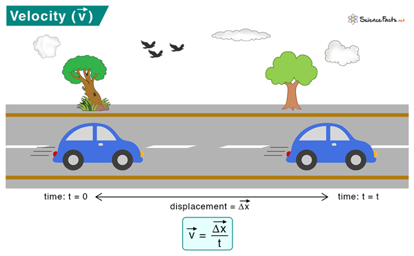
Velocity is the rate at which an object changes position with time. An object is displaced when it changes its position. The amount of displacement over the time in which the displacement occurred gives the velocity. It is a vector quantity that has both magnitude and direction.

The importance of velocity is that it can give you an estimated time to go from one point to another. Suppose you are traveling from place A to place B. Velocity tells you how long it will take to arrive at your destination.

How to Calculate Velocity

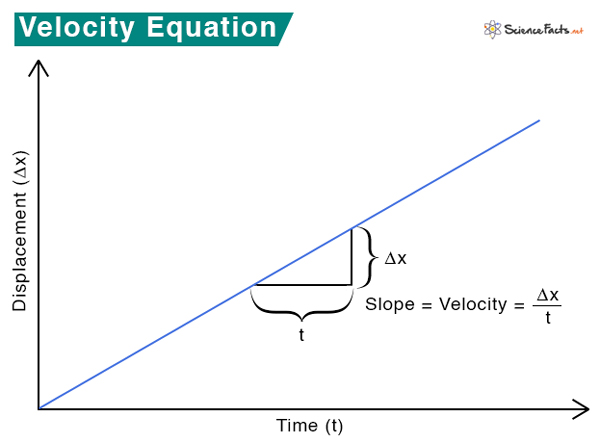
Velocity can be calculated by measuring the object’s displacement over the time taken to displace it.

In vectorial notation, velocity is given by

The SI unit of velocity is Newtons per second of N/s. The cgs unit is ergs per second or ergs/s. Other units include miler per hour or mph, kilometers per hour or kph, and feet per second or fps.

A car traveling on the highway at 60 mph toward the West
A biker riding on the road at 35 mph toward the southwest
A bicyclist heading northwards at 14 mph
An airplane flying eastwards at 300 mph
A rocket launched into the sky in the south-east direction
A train traveling in the south direction at 80 kph
A runner runs 420 m in 70 seconds

Average and Instantaneous Velocity

An object can move from one position to another in several steps. The average velocity is simply the change in position over the time interval within which change takes place.

v avg is the average velocity

x f is the final velocity

x i is the initial velocity

t f is the final time

t i is the initial time

If the starting time is zero, then t i = 0.

The instantaneous (v ins. ) velocity is the velocity at a particular instant of time. It can be obtained by taking the limit of the above expression in the limit Δt → 0.

Speed vs. Velocity

Both speed and velocity measure rate. Both of them depict how fast an object is moving. However, there is an essential difference. While speed tells us the magnitude of the rate at which the object moves, it does not say anything about the direction. On the other hand, velocity considers the direction of motion.

Let us take an example to illustrate this. When we say a car is moving on the road at 35 mph, we specify the magnitude but not the direction. However, when we say a car is moving on the road eastwards at 35 mph, we specify both the magnitude and direction. The first sentence refers to the speed, and the second refers to the velocity. Therefore, speed is a scalar quantity, and velocity is a vector quantity.

The formula for speed is the distance traveled over the time taken to travel that distance.

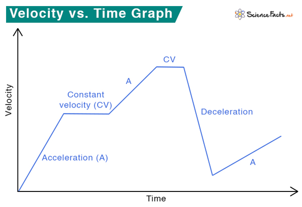
Velocity vs. Time Graph

The following graph shows how velocity changes with time. At some parts of the graph, the velocity increases linearly with time. The quotient of velocity and time is called acceleration . When the velocity decreases with time, the phenomenon is known as deceleration. Regions of constant velocity are also indicated on the graph.

Solved Problems

Problem 1. Suppose a runner moves along the x-direction over some time.During a 5.00 s interval, the runner’s position changes from x 1 = 75 m to x 2 = 35 m. What was the runner’s average velocity?

Given x 1 = 75 m, x 2 = 35 m, Δt = 5 s

The average velocity is given by

v avg = (x 2 – x 1 )/Δt = (35 m – 75 m)/5s = – 8 m/s

Therefore, the runner is running in the negative x-direction.

Problem 2 . A commuter train travels from New York to Philadelphia in 1 hour and 25 minutes and from Philadelphia to New York in 1 hour and 35 minutes. The distance between the two stations is approximately 96 miles. What is (a) the average velocity of the train and (b) the average speed of the train in m/s? (1 mile = 1.6 km)

a) The average velocity of the train is zero since the displacement is zero. (The train returns to New York).

d = 96 miles = 96 x 1.6 = 153.6 km = 153.6 x 10 3 m

t 1 = 1 hr 25 mins = 60 mins + 25 mins = 85 mins = 85 x 60 = 5100 s

Therefore, v 1 = 153.6 x 10 3 m / 5100 s = 30.2 m/s

t 2 = 1 hr 35 mins = 60 mins + 35 mins = 95 mins = 95 x 60 = 5700 s

Therefore, v 2 = 153.6 x 10 3 m / 5700 s = 26.9 m/s

The average speed is (30.2 m/s + 26.9 m/s)/2 = 28.55 m/s

Speed vs. Velocity – Physicsclassroom.com
What is Velocity? – Khanacademy.org
What is Velocity in Physics? – Thoughtco.com
Speed and Velocity – Physics.info
Instantaneous Velocity and Speed – Pressbooks.online.ucf.edu
Time, Velocity, and Speed – Phys.libretexts.org
Velocity – Hyperphysics.phy-astr.gsu.edu

Article was last reviewed on Friday, July 28, 2023

2 responses to “Velocity”

on concept of vector

A vector is a physical quantity that has both magnitude and direction.

Join our Newsletter

Fill your E-mail Address

Related Worksheets

TPC and eLearning
What's NEW at TPC?
Read Watch Interact
Practice Review Test
Teacher-Tools
Subscription Selection
Seat Calculator
Ad Free Account
Edit Profile Settings
Classes (Version 2)
Student Progress Edit
Task Properties
Export Student Progress
Task, Activities, and Scores
Metric Conversions Questions
Metric System Questions
Metric Estimation Questions
Significant Digits Questions
Proportional Reasoning
Acceleration
Distance-Displacement
Dots and Graphs
Graph That Motion
Match That Graph
Name That Motion
Motion Diagrams
Pos'n Time Graphs Numerical
Pos'n Time Graphs Conceptual
Up And Down - Questions
Balanced vs. Unbalanced Forces
Change of State
Force and Motion
Mass and Weight
Match That Free-Body Diagram
Net Force (and Acceleration) Ranking Tasks
Newton's Second Law
Normal Force Card Sort
Recognizing Forces
Air Resistance and Skydiving
Solve It! with Newton's Second Law
Which One Doesn't Belong?
Component Addition Questions
Head-to-Tail Vector Addition
Projectile Mathematics
Trajectory - Angle Launched Projectiles
Trajectory - Horizontally Launched Projectiles
Vector Addition
Vector Direction
Which One Doesn't Belong? Projectile Motion
Forces in 2-Dimensions
Being Impulsive About Momentum
Explosions - Law Breakers
Hit and Stick Collisions - Law Breakers
Case Studies: Impulse and Force
Impulse-Momentum Change Table
Keeping Track of Momentum - Hit and Stick
Keeping Track of Momentum - Hit and Bounce
What's Up (and Down) with KE and PE?
Energy Conservation Questions
Energy Dissipation Questions
Energy Ranking Tasks
LOL Charts (a.k.a., Energy Bar Charts)
Match That Bar Chart
Words and Charts Questions
Name That Energy
Stepping Up with PE and KE Questions
Case Studies - Circular Motion
Circular Logic
Forces and Free-Body Diagrams in Circular Motion
Gravitational Field Strength
Universal Gravitation
Angular Position and Displacement
Linear and Angular Velocity
Angular Acceleration
Rotational Inertia
Balanced vs. Unbalanced Torques
Getting a Handle on Torque
Torque-ing About Rotation
Properties of Matter
Fluid Pressure
Buoyant Force
Sinking, Floating, and Hanging
Pascal's Principle
Flow Velocity
Bernoulli's Principle
Balloon Interactions
Charge and Charging
Charge Interactions
Charging by Induction
Conductors and Insulators
Coulombs Law
Electric Field
Electric Field Intensity
Polarization
Case Studies: Electric Power
Know Your Potential
Light Bulb Anatomy
I = ∆V/R Equations as a Guide to Thinking
Parallel Circuits - ∆V = I•R Calculations
Resistance Ranking Tasks
Series Circuits - ∆V = I•R Calculations
Series vs. Parallel Circuits
Equivalent Resistance
Period and Frequency of a Pendulum
Pendulum Motion: Velocity and Force
Energy of a Pendulum
Period and Frequency of a Mass on a Spring
Horizontal Springs: Velocity and Force
Vertical Springs: Velocity and Force
Energy of a Mass on a Spring
Decibel Scale
Frequency and Period
Closed-End Air Columns
Name That Harmonic: Strings
Rocking the Boat
Wave Basics
Matching Pairs: Wave Characteristics
Wave Interference
Waves - Case Studies
Color Addition and Subtraction
Color Filters
If This, Then That: Color Subtraction
Light Intensity
Color Pigments
Converging Lenses
Curved Mirror Images
Law of Reflection
Refraction and Lenses
Total Internal Reflection
Who Can See Who?
Formulas and Atom Counting
Atomic Models
Bond Polarity
Entropy Questions
Cell Voltage Questions
Heat of Formation Questions
Reduction Potential Questions
Oxidation States Questions
Measuring the Quantity of Heat
Hess's Law
Oxidation-Reduction Questions
Galvanic Cells Questions
Thermal Stoichiometry
Molecular Polarity
Quantum Mechanics
Balancing Chemical Equations
Bronsted-Lowry Model of Acids and Bases
Classification of Matter
Collision Model of Reaction Rates
Density Ranking Tasks
Dissociation Reactions
Complete Electron Configurations
Elemental Measures
Enthalpy Change Questions
Equilibrium Concept
Equilibrium Constant Expression
Equilibrium Calculations - Questions
Equilibrium ICE Table
Intermolecular Forces Questions
Ionic Bonding
Lewis Electron Dot Structures
Limiting Reactants
Line Spectra Questions
Mass Stoichiometry
Measurement and Numbers
Metals, Nonmetals, and Metalloids
Metric Estimations
Metric System
Molarity Ranking Tasks
Mole Conversions
Name That Element
Names to Formulas
Names to Formulas 2
Nuclear Decay
Particles, Words, and Formulas
Periodic Trends
Precipitation Reactions and Net Ionic Equations
Pressure Concepts
Pressure-Temperature Gas Law
Pressure-Volume Gas Law
Chemical Reaction Types
Significant Digits and Measurement
States Of Matter Exercise
Stoichiometry Law Breakers
Stoichiometry - Math Relationships
Subatomic Particles
Spontaneity and Driving Forces
Gibbs Free Energy
Volume-Temperature Gas Law
Acid-Base Properties
Energy and Chemical Reactions
Chemical and Physical Properties
Valence Shell Electron Pair Repulsion Theory
Writing Balanced Chemical Equations
Mission CG1
Mission CG10
Mission CG2
Mission CG3
Mission CG4
Mission CG5
Mission CG6
Mission CG7
Mission CG8
Mission CG9
Mission EC1
Mission EC10
Mission EC11
Mission EC12
Mission EC2
Mission EC3
Mission EC4
Mission EC5
Mission EC6
Mission EC7
Mission EC8
Mission EC9
Mission RL1
Mission RL2
Mission RL3
Mission RL4
Mission RL5
Mission RL6
Mission KG7
Mission RL8
Mission KG9
Mission RL10
Mission RL11
Mission RM1
Mission RM2
Mission RM3
Mission RM4
Mission RM5
Mission RM6
Mission RM8
Mission RM10
Mission LC1
Mission RM11
Mission LC2
Mission LC3
Mission LC4
Mission LC5
Mission LC6
Mission LC8
Mission SM1
Mission SM2
Mission SM3
Mission SM4
Mission SM5
Mission SM6
Mission SM8
Mission SM10
Mission KG10
Mission SM11
Mission KG2
Mission KG3
Mission KG4
Mission KG5
Mission KG6
Mission KG8
Mission KG11
Mission F2D1
Mission F2D2
Mission F2D3
Mission F2D4
Mission F2D5
Mission F2D6
Mission KC1
Mission KC2
Mission KC3
Mission KC4
Mission KC5
Mission KC6
Mission KC7
Mission KC8
Mission AAA
Mission SM9
Mission LC7
Mission LC9
Mission NL1
Mission NL2
Mission NL3
Mission NL4
Mission NL5
Mission NL6
Mission NL7
Mission NL8
Mission NL9
Mission NL10
Mission NL11
Mission NL12
Mission MC1
Mission MC10
Mission MC2
Mission MC3
Mission MC4
Mission MC5
Mission MC6
Mission MC7
Mission MC8
Mission MC9
Mission RM7
Mission RM9
Mission RL7
Mission RL9
Mission SM7
Mission SE1
Mission SE10
Mission SE11
Mission SE12
Mission SE2
Mission SE3
Mission SE4
Mission SE5
Mission SE6
Mission SE7
Mission SE8
Mission SE9
Mission VP1
Mission VP10
Mission VP2
Mission VP3
Mission VP4
Mission VP5
Mission VP6
Mission VP7
Mission VP8
Mission VP9
Mission WM1
Mission WM2
Mission WM3
Mission WM4
Mission WM5
Mission WM6
Mission WM7
Mission WM8
Mission WE1
Mission WE10
Mission WE2
Mission WE3
Mission WE4
Mission WE5
Mission WE6
Mission WE7
Mission WE8
Mission WE9
Vector Walk Interactive
Name That Motion Interactive
Kinematic Graphing 1 Concept Checker
Kinematic Graphing 2 Concept Checker
Graph That Motion Interactive
Two Stage Rocket Interactive
Rocket Sled Concept Checker
Force Concept Checker
Free-Body Diagrams Concept Checker
Free-Body Diagrams The Sequel Concept Checker
Skydiving Concept Checker
Elevator Ride Concept Checker
Vector Addition Concept Checker
Vector Walk in Two Dimensions Interactive
Name That Vector Interactive
River Boat Simulator Concept Checker
Projectile Simulator 2 Concept Checker
Projectile Simulator 3 Concept Checker
Hit the Target Interactive
Turd the Target 1 Interactive
Turd the Target 2 Interactive
Balance It Interactive
Go For The Gold Interactive
Egg Drop Concept Checker
Fish Catch Concept Checker
Exploding Carts Concept Checker
Collision Carts - Inelastic Collisions Concept Checker
Its All Uphill Concept Checker
Stopping Distance Concept Checker
Chart That Motion Interactive
Roller Coaster Model Concept Checker
Uniform Circular Motion Concept Checker
Horizontal Circle Simulation Concept Checker
Vertical Circle Simulation Concept Checker
Race Track Concept Checker
Gravitational Fields Concept Checker
Orbital Motion Concept Checker
Angular Acceleration Concept Checker
Balance Beam Concept Checker
Torque Balancer Concept Checker
Aluminum Can Polarization Concept Checker
Charging Concept Checker
Name That Charge Simulation
Coulomb's Law Concept Checker
Electric Field Lines Concept Checker
Put the Charge in the Goal Concept Checker
Circuit Builder Concept Checker (Series Circuits)
Circuit Builder Concept Checker (Parallel Circuits)
Circuit Builder Concept Checker (∆V-I-R)
Circuit Builder Concept Checker (Voltage Drop)
Equivalent Resistance Interactive
Pendulum Motion Simulation Concept Checker
Mass on a Spring Simulation Concept Checker
Particle Wave Simulation Concept Checker
Boundary Behavior Simulation Concept Checker
Slinky Wave Simulator Concept Checker
Simple Wave Simulator Concept Checker
Wave Addition Simulation Concept Checker
Standing Wave Maker Simulation Concept Checker
Color Addition Concept Checker
Painting With CMY Concept Checker
Stage Lighting Concept Checker
Filtering Away Concept Checker
InterferencePatterns Concept Checker
Young's Experiment Interactive
Plane Mirror Images Interactive
Who Can See Who Concept Checker
Optics Bench (Mirrors) Concept Checker
Name That Image (Mirrors) Interactive
Refraction Concept Checker
Total Internal Reflection Concept Checker
Optics Bench (Lenses) Concept Checker
Kinematics Preview
Velocity Time Graphs Preview
Moving Cart on an Inclined Plane Preview
Stopping Distance Preview
Cart, Bricks, and Bands Preview
Fan Cart Study Preview
Friction Preview
Coffee Filter Lab Preview
Friction, Speed, and Stopping Distance Preview
Up and Down Preview
Projectile Range Preview
Ballistics Preview
Juggling Preview
Marshmallow Launcher Preview
Air Bag Safety Preview
Colliding Carts Preview
Collisions Preview
Engineering Safer Helmets Preview
Push the Plow Preview
Its All Uphill Preview
Energy on an Incline Preview
Modeling Roller Coasters Preview
Hot Wheels Stopping Distance Preview
Ball Bat Collision Preview
Energy in Fields Preview
Weightlessness Training Preview
Roller Coaster Loops Preview
Universal Gravitation Preview
Keplers Laws Preview
Kepler's Third Law Preview
Charge Interactions Preview
Sticky Tape Experiments Preview
Wire Gauge Preview
Voltage, Current, and Resistance Preview
Light Bulb Resistance Preview
Series and Parallel Circuits Preview
Thermal Equilibrium Preview
Linear Expansion Preview
Heating Curves Preview
Electricity and Magnetism - Part 1 Preview
Electricity and Magnetism - Part 2 Preview
Vibrating Mass on a Spring Preview
Period of a Pendulum Preview
Wave Speed Preview
Slinky-Experiments Preview
Standing Waves in a Rope Preview
Sound as a Pressure Wave Preview
DeciBel Scale Preview
DeciBels, Phons, and Sones Preview
Sound of Music Preview
Shedding Light on Light Bulbs Preview
Models of Light Preview
Electromagnetic Radiation Preview
Electromagnetic Spectrum Preview
EM Wave Communication Preview
Digitized Data Preview
Light Intensity Preview
Concave Mirrors Preview
Object Image Relations Preview
Snells Law Preview
Reflection vs. Transmission Preview
Magnification Lab Preview
Reactivity Preview
Ions and the Periodic Table Preview
Periodic Trends Preview
Chemical Reactions Preview
Intermolecular Forces Preview
Melting Points and Boiling Points Preview
Bond Energy and Reactions Preview
Reaction Rates Preview
Ammonia Factory Preview
Stoichiometry Preview
Nuclear Chemistry Preview
Gaining Teacher Access
Tasks and Classes
Tasks - Classic
Subscription
Subscription Locator
1-D Kinematics
Newton's Laws
Vectors - Motion and Forces in Two Dimensions
Momentum and Its Conservation
Work and Energy
Circular Motion and Satellite Motion
Thermal Physics
Static Electricity
Electric Circuits
Vibrations and Waves
Sound Waves and Music
Light and Color
Reflection and Mirrors
About the Physics Interactives
Task Tracker
Usage Policy
Newtons Laws
Vectors and Projectiles
Forces in 2D
Momentum and Collisions
Circular and Satellite Motion
Balance and Rotation
Electromagnetism
Waves and Sound
Atomic Physics
Forces in Two Dimensions
Work, Energy, and Power
Circular Motion and Gravitation
Sound Waves
1-Dimensional Kinematics
Circular, Satellite, and Rotational Motion
Einstein's Theory of Special Relativity
Waves, Sound and Light
QuickTime Movies
About the Concept Builders
Pricing For Schools
Directions for Version 2
Measurement and Units
Relationships and Graphs
Rotation and Balance
Vibrational Motion
Reflection and Refraction
Teacher Accounts
Task Tracker Directions
Kinematic Concepts
Kinematic Graphing
Wave Motion
Sound and Music
About CalcPad
1D Kinematics
Vectors and Forces in 2D
Simple Harmonic Motion
Rotational Kinematics
Rotation and Torque
Rotational Dynamics
Electric Fields, Potential, and Capacitance
Transient RC Circuits
Light Waves
Units and Measurement
Stoichiometry
Molarity and Solutions
Thermal Chemistry
Acids and Bases
Kinetics and Equilibrium
Solution Equilibria
Oxidation-Reduction
Nuclear Chemistry
Newton's Laws of Motion
Work and Energy Packet
Static Electricity Review
NGSS Alignments
1D-Kinematics
Projectiles
Circular Motion
Magnetism and Electromagnetism
Graphing Practice
About the ACT
ACT Preparation
For Teachers
Other Resources
Solutions Guide
Solutions Guide Digital Download
Motion in One Dimension
Work, Energy and Power
Algebra Based Physics
Other Tools
Frequently Asked Questions
Purchasing the Download
Purchasing the CD
Purchasing the Digital Download
About the NGSS Corner
NGSS Search
Force and Motion DCIs - High School
Energy DCIs - High School
Wave Applications DCIs - High School
Force and Motion PEs - High School
Energy PEs - High School
Wave Applications PEs - High School
Crosscutting Concepts
The Practices
Physics Topics
NGSS Corner: Activity List
NGSS Corner: Infographics
About the Toolkits
Position-Velocity-Acceleration
Position-Time Graphs
Velocity-Time Graphs
Newton's First Law
Newton's Second Law
Newton's Third Law
Terminal Velocity
Projectile Motion
Forces in 2 Dimensions
Impulse and Momentum Change
Momentum Conservation
Work-Energy Fundamentals
Work-Energy Relationship
Roller Coaster Physics
Satellite Motion
Electric Fields
Circuit Concepts
Series Circuits
Parallel Circuits
Describing-Waves
Wave Behavior Toolkit
Standing Wave Patterns
Resonating Air Columns
Wave Model of Light
Plane Mirrors
Curved Mirrors
Teacher Guide
Using Lab Notebooks
Current Electricity
Light Waves and Color
Reflection and Ray Model of Light
Refraction and Ray Model of Light
Classes (Legacy Version)
Teacher Resources
Subscriptions

Newton's Laws
Einstein's Theory of Special Relativity
About Concept Checkers
School Pricing
Newton's Laws of Motion
Newton's First Law
Newton's Third Law

Kinematic Equations and Problem-Solving

Kinematic Equations Introduction
Solving Problems with Kinematic Equations
Kinematic Equations and Free Fall
Sample Problems and Solutions
Kinematic Equations and Kinematic Graphs

The four kinematic equations that describe the mathematical relationship between the parameters that describe an object's motion were introduced in the previous part of Lesson 6 . The four kinematic equations are:

In the above equations, the symbol d stands for the displacement of the object. The symbol t stands for the time for which the object moved. The symbol a stands for the acceleration of the object. And the symbol v stands for the instantaneous velocity of the object; a subscript of i after the v (as in v i ) indicates that the velocity value is the initial velocity value and a subscript of f (as in v f ) indicates that the velocity value is the final velocity value.

Problem-Solving Strategy

Construct an informative diagram of the physical situation.
Identify and list the given information in variable form.
Identify and list the unknown information in variable form.
Identify and list the equation that will be used to determine unknown information from known information.
Substitute known values into the equation and use appropriate algebraic steps to solve for the unknown information.
Check your answer to insure that it is reasonable and mathematically correct.

The use of this problem-solving strategy in the solution of the following problem is modeled in Examples A and B below.

Example Problem A

Ima Hurryin is approaching a stoplight moving with a velocity of +30.0 m/s. The light turns yellow, and Ima applies the brakes and skids to a stop. If Ima's acceleration is -8.00 m/s 2 , then determine the displacement of the car during the skidding process. (Note that the direction of the velocity and the acceleration vectors are denoted by a + and a - sign.)

The solution to this problem begins by the construction of an informative diagram of the physical situation. This is shown below. The second step involves the identification and listing of known information in variable form. Note that the v f value can be inferred to be 0 m/s since Ima's car comes to a stop. The initial velocity ( v i ) of the car is +30.0 m/s since this is the velocity at the beginning of the motion (the skidding motion). And the acceleration ( a ) of the car is given as - 8.00 m/s 2 . (Always pay careful attention to the + and - signs for the given quantities.) The next step of the strategy involves the listing of the unknown (or desired) information in variable form. In this case, the problem requests information about the displacement of the car. So d is the unknown quantity. The results of the first three steps are shown in the table below.

The next step of the strategy involves identifying a kinematic equation that would allow you to determine the unknown quantity. There are four kinematic equations to choose from. In general, you will always choose the equation that contains the three known and the one unknown variable. In this specific case, the three known variables and the one unknown variable are v f , v i , a , and d . Thus, you will look for an equation that has these four variables listed in it. An inspection of the four equations above reveals that the equation on the top right contains all four variables.

Once the equation is identified and written down, the next step of the strategy involves substituting known values into the equation and using proper algebraic steps to solve for the unknown information. This step is shown below.

(0 m/s) 2 = (30.0 m/s) 2 + 2 • (-8.00 m/s 2 ) • d

0 m 2 /s 2 = 900 m 2 /s 2 + (-16.0 m/s 2 ) • d

(16.0 m/s 2 ) • d = 900 m 2 /s 2 - 0 m 2 /s 2

(16.0 m/s 2 )*d = 900 m 2 /s 2

d = (900 m 2 /s 2 )/ (16.0 m/s 2 )

The solution above reveals that the car will skid a distance of 56.3 meters. (Note that this value is rounded to the third digit.)

The last step of the problem-solving strategy involves checking the answer to assure that it is both reasonable and accurate. The value seems reasonable enough. It takes a car a considerable distance to skid from 30.0 m/s (approximately 65 mi/hr) to a stop. The calculated distance is approximately one-half a football field, making this a very reasonable skidding distance. Checking for accuracy involves substituting the calculated value back into the equation for displacement and insuring that the left side of the equation is equal to the right side of the equation. Indeed it is!

Example Problem B

Ben Rushin is waiting at a stoplight. When it finally turns green, Ben accelerated from rest at a rate of a 6.00 m/s 2 for a time of 4.10 seconds. Determine the displacement of Ben's car during this time period.

Once more, the solution to this problem begins by the construction of an informative diagram of the physical situation. This is shown below. The second step of the strategy involves the identification and listing of known information in variable form. Note that the v i value can be inferred to be 0 m/s since Ben's car is initially at rest. The acceleration ( a ) of the car is 6.00 m/s 2 . And the time ( t ) is given as 4.10 s. The next step of the strategy involves the listing of the unknown (or desired) information in variable form. In this case, the problem requests information about the displacement of the car. So d is the unknown information. The results of the first three steps are shown in the table below.

The next step of the strategy involves identifying a kinematic equation that would allow you to determine the unknown quantity. There are four kinematic equations to choose from. Again, you will always search for an equation that contains the three known variables and the one unknown variable. In this specific case, the three known variables and the one unknown variable are t, v i , a, and d. An inspection of the four equations above reveals that the equation on the top left contains all four variables.

d = (0 m/s) • (4.1 s) + ½ • (6.00 m/s 2 ) • (4.10 s) 2

d = (0 m) + ½ • (6.00 m/s 2 ) • (16.81 s 2 )

d = 0 m + 50.43 m

The solution above reveals that the car will travel a distance of 50.4 meters. (Note that this value is rounded to the third digit.)

The last step of the problem-solving strategy involves checking the answer to assure that it is both reasonable and accurate. The value seems reasonable enough. A car with an acceleration of 6.00 m/s/s will reach a speed of approximately 24 m/s (approximately 50 mi/hr) in 4.10 s. The distance over which such a car would be displaced during this time period would be approximately one-half a football field, making this a very reasonable distance. Checking for accuracy involves substituting the calculated value back into the equation for displacement and insuring that the left side of the equation is equal to the right side of the equation. Indeed it is!

The two example problems above illustrate how the kinematic equations can be combined with a simple problem-solving strategy to predict unknown motion parameters for a moving object. Provided that three motion parameters are known, any of the remaining values can be determined. In the next part of Lesson 6 , we will see how this strategy can be applied to free fall situations. Or if interested, you can try some practice problems and check your answer against the given solutions.

school Campus Bookshelves
menu_book Bookshelves
perm_media Learning Objects
login Login
how_to_reg Request Instructor Account
hub Instructor Commons

Margin Size

Download Page (PDF)
Download Full Book (PDF)
Periodic Table
Physics Constants
Scientific Calculator
Reference & Cite
Tools expand_more
Readability

selected template will load here

This action is not available.

6.3: Solving Problems with Newton's Laws (Part 2)

Last updated
Save as PDF
Page ID 5883

$ \newcommand{\vecs}[1]{\overset { \scriptstyle \rightharpoonup} {\mathbf{#1}} } $

$ \newcommand{\vecd}[1]{\overset{-\!-\!\rightharpoonup}{\vphantom{a}\smash {#1}}} $

$ \newcommand{\id}{\mathrm{id}}$ $ \newcommand{\Span}{\mathrm{span}}$

( \newcommand{\kernel}{\mathrm{null}\,}\) $ \newcommand{\range}{\mathrm{range}\,}$

$ \newcommand{\RealPart}{\mathrm{Re}}$ $ \newcommand{\ImaginaryPart}{\mathrm{Im}}$

$ \newcommand{\Argument}{\mathrm{Arg}}$ $ \newcommand{\norm}[1]{\| #1 \|}$

$ \newcommand{\inner}[2]{\langle #1, #2 \rangle}$

$ \newcommand{\Span}{\mathrm{span}}$

$ \newcommand{\id}{\mathrm{id}}$

$ \newcommand{\kernel}{\mathrm{null}\,}$

$ \newcommand{\range}{\mathrm{range}\,}$

$ \newcommand{\RealPart}{\mathrm{Re}}$

$ \newcommand{\ImaginaryPart}{\mathrm{Im}}$

$ \newcommand{\Argument}{\mathrm{Arg}}$

$ \newcommand{\norm}[1]{\| #1 \|}$

$ \newcommand{\Span}{\mathrm{span}}$ $ \newcommand{\AA}{\unicode[.8,0]{x212B}}$

$ \newcommand{\vectorA}[1]{\vec{#1}} % arrow$

$ \newcommand{\vectorAt}[1]{\vec{\text{#1}}} % arrow$

$ \newcommand{\vectorB}[1]{\overset { \scriptstyle \rightharpoonup} {\mathbf{#1}} } $

$ \newcommand{\vectorC}[1]{\textbf{#1}} $

$ \newcommand{\vectorD}[1]{\overrightarrow{#1}} $

$ \newcommand{\vectorDt}[1]{\overrightarrow{\text{#1}}} $

$ \newcommand{\vectE}[1]{\overset{-\!-\!\rightharpoonup}{\vphantom{a}\smash{\mathbf {#1}}}} $

Newton’s Laws of Motion and Kinematics

Example 6.6: What Force Must a Soccer Player Exert to Reach Top Speed?

A soccer player starts at rest and accelerates forward, reaching a velocity of 8.00 m/s in 2.50 s. (a) What is her average acceleration? (b) What average force does the ground exert forward on the runner so that she achieves this acceleration? The player’s mass is 70.0 kg, and air resistance is negligible.

To find the answers to this problem, we use the problem-solving strategy given earlier in this chapter. The solutions to each part of the example illustrate how to apply specific problem-solving steps. In this case, we do not need to use all of the steps. We simply identify the physical principles, and thus the knowns and unknowns; apply Newton’s second law; and check to see whether the answer is reasonable.

We are given the initial and final velocities (zero and 8.00 m/s forward); thus, the change in velocity is $\Delta$v = 8.00 m/s . We are given the elapsed time, so $\Delta$t = 2.50 s. The unknown is acceleration, which can be found from its definition: $$a = \frac{\Delta v}{\Delta t} \ldotp$$Substituting the known values yields $$a = \frac{8.00\; m/s}{2.50\; s} = 3.20\; m/s^{2} \ldotp$$
Here we are asked to find the average force the ground exerts on the runner to produce this acceleration. (Remember that we are dealing with the force or forces acting on the object of interest.) This is the reaction force to that exerted by the player backward against the ground, by Newton’s third law. Neglecting air resistance, this would be equal in magnitude to the net external force on the player, since this force causes her acceleration. Since we now know the player’s acceleration and are given her mass, we can use Newton’s second law to find the force exerted. That is, $$F_{net} = ma \ldotp$$Substituting the known values of m and a gives $$F_{net} = (70.0\; kg)(3.20\; m/s^{2}) = 224\; N \ldotp$$

This is a reasonable result: The acceleration is attainable for an athlete in good condition. The force is about 50 pounds, a reasonable average force.

Significance

This example illustrates how to apply problem-solving strategies to situations that include topics from different chapters. The first step is to identify the physical principles, the knowns, and the unknowns involved in the problem. The second step is to solve for the unknown, in this case using Newton’s second law. Finally, we check our answer to ensure it is reasonable. These techniques for integrated concept problems will be useful in applications of physics outside of a physics course, such as in your profession, in other science disciplines, and in everyday life.

Exercise 6.4

Example 6.7: What Force Acts on a Model Helicopter?

A 1.50-kg model helicopter has a velocity of 5.00 $\hat{j}$ m/s at t = 0. It is accelerated at a constant rate for two seconds (2.00 s) after which it has a velocity of (6.00 $\hat{i}$ + 12.00 $\hat{j}$) m/s. What is the magnitude of the resultant force acting on the helicopter during this time interval?

We can easily set up a coordinate system in which the x-axis ($\hat{i}$ direction) is horizontal, and the y-axis ($\hat{j}$ direction) is vertical. We know that $\Delta$t = 2.00s and $\Delta$v = (6.00 $\hat{i}$ + 12.00 $\hat{j}$ m/s) − (5.00 $\hat{j}$ m/s). From this, we can calculate the acceleration by the definition; we can then apply Newton’s second law.

\[a = \frac{\Delta v}{\Delta t} = \frac{(6.00 \hat{i} + 12.00 \hat{j}\; m/s) - (5.00 \hat{j}\; m/s)}{2.00\; s} = 3.00 \hat{i} + 3.50 \hat{j}\; m/s^{2}$$ $$\sum \vec{F} = m \vec{a} = (1.50\; kg)(3.00 \hat{i} + 3.50 \hat{j}\; m/s^{2}) = 4.50 \hat{i} + 5.25 \hat{j}\; N \ldotp\]

The magnitude of the force is now easily found:

\[F = \sqrt{(4.50\; N)^{2} + (5.25\; N)^{2}} = 6.91\; N \ldotp\]

The original problem was stated in terms of $\hat{i}$ − $\hat{j}$ vector components, so we used vector methods. Compare this example with the previous example.

Exercise 6.5

Find the direction of the resultant for the 1.50-kg model helicopter.

Example 6.8: Baggage Tractor

Figure $\PageIndex{7}$(a) shows a baggage tractor pulling luggage carts from an airplane. The tractor has mass 650.0 kg, while cart A has mass 250.0 kg and cart B has mass 150.0 kg. The driving force acting for a brief period of time accelerates the system from rest and acts for 3.00 s. (a) If this driving force is given by F = (820.0t) N, find the speed after 3.00 seconds. (b) What is the horizontal force acting on the connecting cable between the tractor and cart A at this instant?

Figure (a) shows a baggage tractor driving to the left and pulling two luggage carts. The external forces on the system are shown. The forces on the tractor are F sub tractor, horizontally to the left, N sub tractor vertically up, and w sub tractor vertically down. The forces on the cart immediately behind the tractor, cart A, are N sub A vertically up, and w sub A vertically down. The forces on cart B, the one behind cart A, are N sub B vertically up, and w sub B vertically down. Figure (b) shows the free body diagram of the tractor, consisting of F sub tractor, horizontally to the left, N sub tractor vertically up, w sub tractor vertically down, and T horizontally to the right.

A free-body diagram shows the driving force of the tractor, which gives the system its acceleration. We only need to consider motion in the horizontal direction. The vertical forces balance each other and it is not necessary to consider them. For part b, we make use of a free-body diagram of the tractor alone to determine the force between it and cart A. This exposes the coupling force $\vec{T}$, which is our objective.

$$\sum F_{x} = m_{system} a_{x}\; and\; \sum F_{x} = 820.0t,$$so $$820.0t = (650.0 + 250.0 + 150.0)a$$ $$a = 0.7809t \ldotp$$Since acceleration is a function of time, we can determine the velocity of the tractor by using a = $\frac{dv}{dt}$ with the initial condition that v 0 = 0 at t = 0. We integrate from t = 0 to t = 3: $$\begin{split}dv & = adt \\ \int_{0}^{3} dv & = \int_{0}^{3.00} adt = \int_{0}^{3.00} 0.7809tdt \\ v & = 0.3905t^{2} \big]_{0}^{3.00} = 3.51\; m/s \ldotp \end{split}$$
Refer to the free-body diagram in Figure $\PageIndex{7}$(b) $$\begin{split} \sum F_{x} & = m_{tractor} a_{x} \\ 820.0t - T & = m_{tractor} (0.7805)t \\ (820.0)(3.00) - T & = (650.0)(0.7805)(3.00) \\ T & = 938\; N \ldotp \end{split}$$

Since the force varies with time, we must use calculus to solve this problem. Notice how the total mass of the system was important in solving Figure $\PageIndex{7}$(a), whereas only the mass of the truck (since it supplied the force) was of use in Figure $\PageIndex{7}$(b).

Recall that v = $\frac{ds}{dt}$ and a = $\frac{dv}{dt}$. If acceleration is a function of time, we can use the calculus forms developed in Motion Along a Straight Line , as shown in this example. However, sometimes acceleration is a function of displacement. In this case, we can derive an important result from these calculus relations. Solving for dt in each, we have dt = $\frac{ds}{v}$ and dt = $\frac{dv}{a}$. Now, equating these expressions, we have $\frac{ds}{v}$ = $\frac{dv}{a}$. We can rearrange this to obtain a ds = v dv.

Example 6.9: Motion of a Projectile Fired Vertically

A 10.0-kg mortar shell is fired vertically upward from the ground, with an initial velocity of 50.0 m/s (see Figure $\PageIndex{8}$). Determine the maximum height it will travel if atmospheric resistance is measured as F D = (0.0100 v 2 ) N, where v is the speed at any instant.

(a) A photograph of a soldier firing a mortar shell straight up. (b) A free body diagram of the mortar shell shows forces F sub D and w, both pointing vertically down. Force w is larger than force F sub D.

The known force on the mortar shell can be related to its acceleration using the equations of motion. Kinematics can then be used to relate the mortar shell’s acceleration to its position.

Initially, y 0 = 0 and v 0 = 50.0 m/s. At the maximum height y = h, v = 0. The free-body diagram shows F D to act downward, because it slows the upward motion of the mortar shell. Thus, we can write

\[\begin{split} \sum F_{y} & = ma_{y} \\ -F_{D} - w & = ma_{y} \\ -0.0100 v^{2} - 98.0 & = 10.0 a \\ a & = -0.00100 v^{2} - 9.80 \ldotp \end{split}\]

The acceleration depends on v and is therefore variable. Since a = f(v), we can relate a to v using the rearrangement described above,

\[a ds = v dv \ldotp\]

We replace ds with dy because we are dealing with the vertical direction,

\[\begin{split} ady & = vdv \\ (−0.00100v^{2} − 9.80)dy & = vdv \ldotp \end{split}\]

We now separate the variables (v’s and dv’s on one side; dy on the other):

\[\begin{split} \int_{0}^{h} dy & = \int_{50.0}^{0} \frac{vdv}{(-0.00100 v^{2} - 9.80)} \\ & = - \int_{50.0}^{0} \frac{vdv}{(-0.00100 v^{2} + 9.80)} \\ & = (-5 \times 10^{3}) \ln(0.00100v^{2} + 9.80) \Big|_{50.0}^{0} \ldotp \end{split}\]

Thus, h = 114 m.

Notice the need to apply calculus since the force is not constant, which also means that acceleration is not constant. To make matters worse, the force depends on v (not t), and so we must use the trick explained prior to the example. The answer for the height indicates a lower elevation if there were air resistance. We will deal with the effects of air resistance and other drag forces in greater detail in Drag Force and Terminal Speed .

Exercise 6.6

If atmospheric resistance is neglected, find the maximum height for the mortar shell. Is calculus required for this solution?

JEE-IIT-NCERT Physics & Math

Widget atas posting, average velocity and average speed problems and solutions.

Problem #1

Acceleration Problems

Search Website

Real World Applications — for high school level and above

Amusement Parks
Battle & Weapons
Engineering
Miscellaneous

Education & Theory — for high school level and above

Useful Formulas
Physics Questions
Example Mechanics Problems
Learn Physics Compendium

Kids Section

Physics For Kids
Science Experiments
Science Fair Ideas
Science Quiz
Science Toys
Teacher Resources
Commercial Disclosure
Privacy Policy

Meta Quest 4
Google Pixel 9
Google Pixel 8a
Apple Vision Pro 2
Nintendo Switch 2
Samsung Galaxy Ring
Yellowstone Season 6
Recall an Email in Outlook
Stranger Things Season 5

Nvidia and Microsoft are solving a big problem with Copilot+

The Surface Laptop running local AI models.

When Microsoft announced Copilot+ PCs a few weeks back, one question reigned supreme : Why can’t I just run these AI applications on my GPU? At Computex 2024 , Nvidia finally provided an answer.

Nvidia and Microsoft are working together on an Application Programming Interface (API) that will allow developers to run their AI-accelerated apps on RTX graphics cards . This includes the various Small Language Models (SLMs) that are part of the Copilot runtime, which are used as the basis for features like Recall and Live Captions.

With the toolkit, developers can allow apps to run locally on your GPU instead of the NPU. This opens up the door to not only more powerful AI applications, as the AI capabilities of GPUs are generally higher than NPUs, but also the ability to run on PCs that don’t currently fall under the Copilot+ umbrella.

It’s a great move. Copilot+ PCs currently require a Neural Processing Unit (NPU) that’s capable of at least 40 Tera Operations Per Second (TOPS). At the moment, only the Snapdragon X Elite satisfies that criteria. Despite that, GPUs have much higher AI processing capabilities, with even low-end models reaching to 100 TOPS, and higher-end options scaling even higher.

In addition to running on the GPU, the new API adds retrieval-augmented generation (RAG) capabilities to the Copilot runtime. RAG gives the AI model access to specific information locally, allowing it to provide more helpful solutions. We saw RAG on full display with Nvidia’s Chat with RTX earlier this year.

Outside of the API, Nvidia announced the RTX AI Toolkit at Computex. This developer suite, arriving in June, combines various tools and SDKs that allow developers to tune AI models for specific applications. Nvidia says that by using the RTX AI Toolkit, developers can make models four times faster and three times smaller compared to using open-source solutions.

We’re seeing a wave of tools that enable developers to build specific AI applications for end users. Some of that is already showing up in Copilot+ PCs, but I suspect we’ll see far more AI applications at this point next year. We have the hardware to run these apps, after all; now we just need the software.

Editors' Recommendations

Intel goes to war with Nvidia and Qualcomm
The Intel we know is dead, but its new Lunar Lake chips are very much alive
Nvidia’s new standard crams an RTX 4080 Super in a tiny case
How to watch Nvidia’s Computex 2024 keynote — and what to expect
Copilot+ was a monster announcement. Here’s how I think Apple will respond

It's not just you -- Microsoft is putting Copilot just about anywhere, and now it's available on Telegram as a bot that's part of its "copilot-for-social" project. Windows Latest reports that to use the bot, you'll need to confirm your phone number by sending your contact in the chat. The company is expanding its AI integration into one of the most popular messaging apps, but it might not end there.

Microsoft claims that it won't save your phone number for anything other than verification, but it's needed because the service is currently unavailable for anyone in the EU, at least for now. If anyone in the EU tries to access it, they will be blocked.

We were just inundated with a whole slew of new Windows laptops. These aren't your average notebooks, though -- they're part of Microsoft's new Copilot+ PC program -- built from the ground up with AI and ARM chips in mind.

A lot of these laptops emphasize the same performance and battery life gains caused by Qualcomm's Snapdragon X chips. Those are impressive, but comparing all these laptops against each other, it's Samsung's entry that makes me the most excited. Design efficiency

Imagine a laptop with an iteration of Nvidia’s ARM-based CPU combined with a powerful RTX graphics card, all enhanced by AI. Years ago, that would have sounded outlandish, but now it seems like it could actually happen.

In a recent interview with Bloomberg, Nvidia CEO Jensen Huang and Dell CEO Michael Dell more or less confirmed that Team Green will enter the AI-PC hype next year.

NXTLVL virtual classroom with individual student video headshots

Problem-Solving Olympiad Puts Power Skills to the Test

The inaugural NXTLVL Problem-Solving Olympiad brought students together online for a day of spirited competition, pushing them to their true potential. Middle school problem-solvers from four continents, including three of the top ten virtual schools ranked by World Schools, navigated complex challenges in teams. These challenges tested timeless Power Skills like creativity, critical thinking, collaboration, communication, emotional intelligence, and resilience.

NXTLVL is a pioneering edtech program that helps students develop Power Skills, preparing them for a rapidly evolving world driven by AI advancements and scientific innovations. Our game-based learning approach combines team challenges with expert coaching, equipping students with the skills needed to take on anything.

Many progressive schools, like those attending the Olympiad, are integrating competency-based education into their curricula, focusing on Power Skills to prepare their students for school, work and life.

Gabriel Hernandez, Director of Technology at our champion school Alverno Heights Academy believes “participation in such interactive activities not only enriches students’ learning experiences but also helps them develop essential skills that are beneficial for their personal and academic growth.”

The new Problem-Solving Olympiad offers an extraordinary learning environment for tomorrow’s problem-solvers to stretch their Power Skills by collaborating under pressure.

Schools from around the world took on the May Olympiad. Photo provided by NXTLVL.

Power Skill award winners

To emphasize the importance of Power Skills, we rewarded exceptional examples.

The Emotional Intelligence Award went to Minerva’s Virtual Academy, a globally recognized online school based in the UK, for “anticipating the needs and strategies of allies and opponents to navigate conflicts.”

Williamsburg Academy of Colorado picked up the Resilience Award for “perseverance in pushing through setbacks without losing momentum.”

Laurel Springs School earned the Critical Thinking Award for “demonstrating exceptional analytical thinking, decoding complex problems with logical and strategically sound solutions.”

The Communication and Creativity Awards went to the Prisma Online School for “mastering divergent thinking, consistently generating and synthesizing innovative ideas, while communicating them clearly.”

The Power Skills Awards. Photo provided by NXTLVL.

The Champions

We witnessed the peak of escalating intensity in the Championship Level as four teams battled it out for the main prize. Fourth place went to Prisma Online School, third place to Hill Top Preparatory School, and second place to Minerva’s Virtual Academy.

Our overall champions were a team from Alverno Heights Academy, an independent Catholic school from California. They epitomized teamwork, securing the Power Skill Award for collaboration. With a perfect balance of leadership and emotional intelligence, they leveraged each other’s diverse skills and perspectives. Their dynamism and synchronicity were evident from start to finish. Worthy winners indeed.

Hernandez added, “This Olympiad provides a unique platform for students to engage in communication and critical thinking skills, which are essential in today’s educational landscape. While traditional sports often focus on teamwork and collaboration, this competition allows educators to reach a broader spectrum of students and foster these important skills collectively.”

One of the Alverno Heights Academy students emphasized the importance of “teamwork, communication, and lots of planning before each round,” which was key to their success.

The 6 Power Skills trophies sit inside the champions’ trophy. Photo provided by NXTLVL.

The ultimate contest of wits

The Olympiad was a breathtaking experience. The speed at which all teams adapted to the surmounting challenges reminded us of what students are capable of when given the right platform. In just five hours, students transformed from being curious but uncertain to astute problem-solving teams.

Initially, they dove in without knowing the rules, requiring them to decode the game, develop hypotheses, and fine-tune their tactics. As the game evolved, they had to rework their strategies and adapt on the fly. This journey through failure, setbacks, and upended strategies led them to a finish line where the sweetness of victory was palpable.

The next level

Building on the success of the May event, we’re excited to announce the November Olympiad, which promises to be even more spectacular, expanding over multiple days to welcome more schools.

With early bird access, it’s free for the first four teams until July 1st.

Click here to register and give your students a head start on the future.

We extend a heartfelt thank you to the Elite Academic Academy for their invaluable support in hosting the event and the other schools that made it possible.

Alverno Heights Academy Boston College High School Colégio Bento Benedini Hill Top Preparatory School Laurel Springs School Leadership Academy of Utah Mesa Public Schools Minerva’s Virtual Academy Prisma Online School Repton Abu Dhabi Repton Al Barsha Repton Dubai Williamsburg Academy Williamsburg Academy of Colorado

Sign Up for EdWeek Tech Leader

From Collective Conflict to Collaborative Problem Solving: Unraveling the Knots of Perception to Solve Functional Problems

This session uncovers the nuanced distinction between conflicts, (which often arise from subjective perspectives and perception misalignments such as patient-provider conflicts, nurse-doctor conflicts, etc., that obscure the underlying, objective challenges that teams face) and functional problems within any multidisciplinary effort. Join two experts explore how to transform conflict into a catalyst for uncovering and addressing the core issues at hand by understanding the nature of conflict and employing practical frameworks.

Learning Objectives:

Understand the nature of conflict and functional problems, gain insight into the psychological underpinnings of conflicts and how they differ from objective, functional problems and identify the heart of collective challenges, moving beyond subjective disagreements.
Leverage conflict for collaborative problem-solving, learn to apply principles and tools to harness conflict constructively and discover how to use conflicts as a focus area to address and solve underlying functional problems, leading to enhanced team cohesion, satisfaction and productivity.
Learn how to shift focus from individual disagreements to collaborative problem-solving, fostering a culture of engagement and shared success.

Brian R. Spisak, PhD , independent consultant; research associate, National Preparedness Leadership Initiative, Harvard University; ACHE Faculty

Rick van Pelt, MD chief clinical transformation officer, leader of the Clinical Practice Transformation Department, University of Alabama at Birmingham Medicine

Cancellation:

To cancel your webinar registration, please notify the Customer Service Center, at [email protected] , at least two business days before the start of the webinar for a refund or credit. After that time, a refund or credit is forfeited.

Continuing Education Credit

Ache qualifying education credit.

This webinar is eligible for 1 ACHE Qualifying Education credit. ACHE Qualifying Education credits will be automatically updated in your My ACHE account upon completion of the recording.

Interprofessional Continuing Education Credit

In support of improving patient care, the American College of Healthcare Executives is jointly accredited by the Accreditation Council for Continuing Medical Education (ACCME), the Accreditation Council for Pharmacy Education (ACPE), the American Nurses Credentialing Center (ANCC), and the American Academy of PAs (AAPA) to provide continuing education for the healthcare team.

This activity was planned by and for the healthcare team, and learners will receive a maximum of 1 Interprofessional Continuing Education (IPCE) credit for learning and change. For further information about Joint Accreditation credits and certificates, please click here .

Physician Continuing Medical Education

The American College of Healthcare Executives (ACHE) designates this live activity for a maximum of 1 AMA PRA Category 1 Credits ™ . Physicians should claim only the credit commensurate with the extent of their participation in the activity.

Continuing Nursing Education

The American College of Healthcare Executives designates this live activity for a maximum of 1 contact hours of continuing nursing education.

Continuing Pharmacy Education

The American College of Healthcare Executives designates this knowledge-based activity for a maximum 1 contact hours of continuing pharmacy education credit.

Continuing Social Work Education

The American College of Healthcare Executives designates this knowledge-based activity for a maximum 1 contact hours of continuing social work education credit.

Continuing Education for Dietitians

The American College of Healthcare Executives designates this knowledge-based activity for a maximum 1 contact hours of continuing education credit for Registered Dietitians and Dietetic Technicians, Registered. RDs and DTRs should enter activities offered by jointly accredited providers as type 102 on Professional Development Portfolio (PDP) activity logs. CPEUs awarded must be commensurate with participation in the activity.

Physician Associate/Physician Assistant Continuing Education

The American College of Healthcare Executives has been authorized by the American Academy of PAs (AAPA) to award AAPA Category 1 CME credit for activities planned in accordance with AAPA CME Criteria. This activity is designated for a maximum of 1 AAPA Category 1 CME credits. PAs should only claim credit commensurate with the extent of their participation.

Surprise eyeing 2,000 acres along McMicken Dam for open space, parks

By 2030, Surprise wants roughly 850 acres of open space available for residents and visitors to enjoy recreationally.

To reach that goal, it’s been eyeing 2,000 acres along the McMicken Dam, where it looks to establish a preserve that includes areas for parks, wildlife corridors and hiking and biking trails.

First, the city must partner with the Maricopa County Flood Control District, the owner of the roughly 14-mile-long structure that divides Surprise between its largely developed half in the southeast and its vacant land in the northwest.

Under a joint-use agreement the city wants to secure with county leaders in the coming years, Surprise could manage and maintain the swath of desert west of Loop 303, between Peoria and Grand avenues.

It would run through the heart of the city.

“This would be very much at the center of the city with this large open space greenway and potential corridor project,” Strategic Initiatives Director Eric Fitzer told city leaders last month, noting the city’s anticipated growth to the north and west of the dam.

What is the city planning to do with the land?

If Surprise partners with the Flood Control District, the city intends to conserve most of the land, keeping it as open space.

The southernmost portion of the land, stretching out of the White Tank Mountain Regional Park, would be maintained as a wildlife corridor, where animals like javelina and mule deer can continue to roam.

Other parts of the land will provide opportunities to develop recreational areas.

“Every city needs a vast amount of open space and parks associated with it, as well as to preserve those areas for the usage and enjoyment of our citizens,” Fitzer told The Arizona Republic last week.

A 13-mile stretch of the Maricopa Trail — the 315-mile-long path looping around the Valley — runs along McMicken Dam in Surprise.

The city wants to expand on those trails, creating more opportunities for hikers and bicyclists, Fitzer said.

There are also areas where the city could develop parks.

One would potentially fit around the Maricopa Trail’s Sun Valley Trailhead, where Bell Road turns into Sun Valley Parkway.

A portion of the land south of Grand Avenue could also be used for a regional park. The city, Fitzer said, is looking at public-private partnerships to develop the concept. Such a park could include amenities like sports fields.

What responsibilities would Surprise have?

As part of the potential joint-use agreement, the city is committed to maintaining the land around McMicken Dam, while Flood Control maintains oversight of the structure.

The city’s responsibilities include cleaning up the desert, making sure people don’t illegally dump trash, and mending broken fences, among other things.

Based on estimates the county provided Surprise, the city anticipates spending about $200,000 to $300,000 annually on maintenance, Fitzer said.

“We don’t foresee a lot (of maintenance) but just in case, there is going to be some allocation for that,” he said.

Asked whether such maintenance would require additional staff, Fitzer noted that the city doesn’t anticipate needing more employees.

“But that’s always a possibility,” he acknowledged.

Whether the land would require a lot of water, Fitzer said that’s unlikely.

“It would be a preserve, so we don’t use a lot of water in this area,” he said. “However, if some of the regional parks potentially are foreseen then at that point there would need to be water allocated out there.”

Solving the Surprise’s open space problem

While Surprise has more than 300 acres of developed parks , it doesn’t own any land designated as open space.

The potential joint-use agreement looks to resolve that.

It would also help the city reach a goal outlined in its 2015 Parks and Recreation Master Plan , a living document meant to guide officials’ and leaders’ decisions about new and existing parks.

In it, the city set out to have 847 acres of open space in its inventory of recreational areas by 2030, when Surprise’s population is estimated to reach 234,579.

The open space concept, Councilmember Chris Judd said during the May 21 meeting, would be something for residents to “truly enjoy.”

“This really positions us well going into the future to sort of handle our open space problems,” he said.

What’s next?

Surprise officials will continue discussions with Flood Control to establish a partnership, Fitzer said.

According to him, getting the joint-use agreement going is about a one- to two-year process. The agreement itself would require approval from both the Surprise City Council and the Maricopa County Board of Supervisors.

Shawn Raymundo covers the West Valley cities of Glendale, Peoria and Surprise. Reach him at [email protected] or follow him on X @ShawnzyTsunami.

A PINN-based level-set formulation for reconstruction of bubble dynamics

Published: 30 May 2024

Cite this article

Rômulo M. Silva 1 na1 ,
Malú Grave 2 na1 &
Alvaro L. G. A. Coutinho 1 na1

90 Accesses

Explore all metrics

Solving problems in fluid mechanics plays an essential role in science and engineering, especially when it comes to optimal design, reconstruction of biomedical and geophysical flows, parameter estimation, and more. In some of these problems, only part of the data (or parameters) are known, and they fall within the broad categories of inverse and mixed problems. Thus, solving them using traditional methods is challenging or sometimes even impossible. Moreover, generating simulated data for such problems can become very costly since simulations need to be performed several times to either discover missing physics or calibrate the free parameters in the model. One possible alternative for overcoming these drawbacks is through the use of Physics-Informed Neural Networks—PINNs, in which we approximate the problem’s solution using neural networks (NNs) while incorporating the known data and physical laws when training it and also easily enabling us to take advantage of computational resources like GPUs. Here, we show a Level-Set PINN-based framework for reconstructing the velocity field for bubble flows. Given only the bubble position, we apply the framework to reconstruct gas bubbles rising in viscous liquid problems. We use synthetic data generated by adaptive mesh refinement and coarsening simulations with a different method, a phase-field approach. The only data provided is a set of snapshots containing the bubble position, i.e., the phase field, from which we try to infer the velocities. Our approach does not require any reinitialization scheme, as is usual when using a level-set approach and traditional numerical methods. Such a scheme can reconstruct the flow quantities with reasonable accuracy, and it is straightforward to parallelize when using a data-parallel approach.

This is a preview of subscription content, log in via an institution to check access.

Access this article

Price includes VAT (Russian Federation)

Instant access to the full article PDF.

Rent this article via DeepDyve

Institutional subscriptions

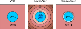
Scientific Machine Learning Through Physics–Informed Neural Networks: Where we are and What’s Next

Physics-informed neural networks (PINNs) for fluid mechanics: a review

Threshold Pressure in Non-Darcian Flow Derived from the Langevin Equation and Fluctuation Dissipation Theorem: Generalized Darcy’s Law

Code availability.

The authors will make the code available upon request if the paper is accepted.

Raissi, M., Perdikaris, P., Karniadakis, G.E.: Physics-informed neural networks: a deep learning framework for solving forward and inverse problems involving nonlinear partial differential equations. J. Comput. Phys. 378 , 686–707 (2019)

Article MathSciNet Google Scholar

Hennigh, O., Narasimhan, S., Nabian, M.A., Subramaniam, A., Tangsali, K., Fang, Z., Rietmann, M., Byeon, W., Choudhry, S.: NVIDIA SimNetTM: An AI-Accelerated Multi-Physics Simulation Framework. In: Paszynski, M., Kranzlmüller, D., Krzhizhanovskaya, V.V., Dongarra, J.J., Sloot, P.M.A (eds.) Computational Science – ICCS 2021, pp. 447–461. Springer International Publishing, Cham (2021). https://doi.org/10.1007/978-3-030-77977-1_36

Kurth, T., Subramanian, S., Harrington, P., Pathak, J., Mardani, M., Hall, D., Miele, A., Kashinath, K., Anandkumar, A.: FourCastNet: Accelerating Global High-Resolution Weather Forecasting Using Adaptive Fourier Neural Operators. Association for Computing Machinery, New York, NY, USA (2023). https://doi.org/10.1145/3592979.3593412

Raissi, M., Yazdani, A., Karniadakis, G.E.: Hidden fluid mechanics: learning velocity and pressure fields from flow visualizations. Science 367 (6481), 1026–1030 (2020)

Lu, L., Meng, X., Mao, Z., Karniadakis, G.E.: Deepxde: a deep learning library for solving differential equations. SIAM Rev. 63 (1), 208–228 (2021)

Lu, L., Jin, P., Pang, G., Zhang, Z., Karniadakis, G.E.: Learning nonlinear operators via DeepONet based on the universal approximation theorem of operators. Nat. Mach. Intell. 3 (3), 218–229 (2021)

Article Google Scholar

Li, Z., Kovachki, N., Azizzadenesheli, K., Liu, B., Bhattacharya, K., Stuart, A. Anandkumar, A.: Fourier neural operator for parametric partial differential equations (2020)

Seidman, J., Kissas, G., Perdikaris, P., Pappas, G.J.: NOMAD: nonlinear manifold decoders for operator learning. Adv. Neural. Inf. Process. Syst. 35 , 5601–5613 (2022)

Google Scholar

Kissas, G., Seidman, J.H., Guilhoto, L.F., Preciado, V.M., Pappas, G.J., Perdikaris, P.: Learning operators with coupled attention. J. Mach. Learn. Res. 23 (215), 1–63 (2022)

MathSciNet Google Scholar

Aldirany, Z., Cottereau, R., Laforest, M., Prudhomme, S.: Approximating the operator of the wave equation using deep learning. 11 (2022)

Margossian, C.C.: A review of automatic differentiation and its efficient implementation. Wiley Interdiscip. Rev. Data Mining Knowl. Discov. 9 (4), e1305 (2019)

Lagaris, I.E., Likas, A., Fotiadis, D.I.: Artificial neural networks for solving ordinary and partial differential equations. IEEE Trans. Neural Netw. 9 (5), 987–1000 (1998)

Kharazmi, E., Zhang, Z., Karniadakis, G.E.: hp-VPINNs: variational physics-informed neural networks with domain decomposition. Comput. Methods Appl. Mech. Eng. 374 , 113547 (2021)

Yang, L., Meng, X., Karniadakis, G.E.: B-PINNs: Bayesian physics-informed neural networks for forward and inverse PDE problems with noisy data. J. Comput. Phys. 425 , 109913 (2021)

Yang, L., Zhang, D., Karniadakis, G.E.: Physics-informed generative adversarial networks for stochastic differential equations. SIAM J. Sci. Comput. 42 (1), A292–A317 (2020)

Daw, A., Maruf, M., Karpatne, A.: PID-GAN: A GAN framework based on a physics-informed discriminator for uncertainty quantification with physics. In: Proceedings of the 27th ACM SIGKDD Conference on Knowledge Discovery & Data Mining, KDD ’21, pp 237–247, New York, NY, USA. Association for Computing Machinery (2021)

Pang, G., D’Elia, M., Parks, M., Karniadakis, G.E.: nPINNs: nonlocal physics-informed neural networks for a parametrized nonlocal universal Laplacian operator algorithms and applications. J. Comput. Phys. 422 , 109760 (2020)

Jagtap, A.D., Kharazmi, E., Karniadakis, G.E.: Conservative physics-informed neural networks on discrete domains for conservation laws: applications to forward and inverse problems. Comput. Methods Appl. Mech. Eng. 365 , 113028 (2020)

Jagtap, A., Karniadakis, G.: Extended physics-informed neural networks (XPINNs): a generalized space-time domain decomposition based deep learning framework for nonlinear partial differential equations. Commun. Comput. Phys. 28 (5), 2002–2041 (2020)

Shukla, K., Jagtap, A.D., Karniadakis, G.E.: Parallel physics-informed neural networks via domain decomposition. J. Comput. Phys. 447 , 110683 (2021)

Daw, A., Bu, J.,Wang, S., Perdikaris, P., Karpatne, A.: Mitigating propagation failures in physics-informed neural networks using retain-resample-release (r3) sampling. In: Proceedings of the 40th International Conference on Machine Learning. Honolulu, Hawaii, USA (2023)

Gao, W., Wang, C.: Active learning based sampling for high-dimensional nonlinear partial differential equations. J. Comput. Phys. 475 , 111848 (2023)

Subramanian, S., Kirby, R.M., Mahoney, M.W., Gholami, A.: Adaptive self-supervision algorithms for physics-informed neural networks (2022)

Tang, K., Wan, X., Yang, C.: DAS-PINNs: a deep adaptive sampling method for solving high-dimensional partial differential equations. J. Comput. Phys. 476 , 111868 (2023)

Chenxi, W., Zhu, M., Tan, Q., Kartha, Y., Lu, L.: A comprehensive study of non-adaptive and residual-based adaptive sampling for physics-informed neural networks. Comput. Methods Appl. Mech. Eng. 403 , 115671 (2023)

Bu, J., Karpatne, A.: Quadratic residual networks: A new class of neural networks for solving forward and inverse problems in physics involving pdes. In: Proceedings of the 2021 SIAM International Conference on Data Mining (SDM), pp. 675–683 (2021)

Wang, S., Wang, H., Seidman, J.H., Perdikaris, P.: Random weight factorization improves the training of continuous neural representations (2022). arXiv:2210.01274

Sitzmann, V., Martel, J., Bergman, A., Lindell, D., Wetzstein, G.: Implicit neural representations with periodic activation functions. Adv. Neural Inf. Process. Syst. 33 , 7462–7473 (2020)

Jagtap, A.D., Kawaguchi, K., Karniadakis, G.E.: Adaptive activation functions accelerate convergence in deep and physics-informed neural networks. J. Comput. Phys. 404 , 109136 (2020)

Cuomo, S., Di Cola, V.S., Giampaolo, F., Rozza, G., Raissi, M., Piccialli, F.: Scientific machine learning through physics-informed neural networks: where we are and what’s next. J. Sci. Comput. 92 (3), 88 (2022)

Cai, S., Wang, Z., Wang, S., Perdikaris, P., Karniadakis, G.E.: Physics-informed neural networks for heat transfer problems. J. Heat Transf. 143 (6), 060801 (2021)

Faroughi, S.A., Pawar, N., Fernandes, C., Raissi, M., Das, S., Kalantari, N.K. Mahjour, S.K.: Physics-guided, physics-informed, and physics-encoded neural networks in scientific computing (2022)

Willard, J., Jia, X., Xu, S., Steinbach, M., Kumar, V.: Integrating scientific knowledge with machine learning for engineering and environmental systems. ACM Comput. Surv. 55 (4), 1–37 (2022)

Brunton, S.L., Kutz, J.N.: Data-Driven Science and Engineering: Machine Learning, Dynamical Systems, and Control, 2nd edn. Cambridge University Press, Cambridge (2022)

Book Google Scholar

Thuerey, N., Holl, P., Mueller, M., Schnell, P., Trost, F., Um, K.: Physics-based Deep Learning. WWW (2021). https://physicsbaseddeeplearning.org

Cai, S., Wang, Z., Fuest, F., Jeon, Y.J., Gray, C., Karniadakis, G.E.: Flow over an espresso cup: inferring 3-D velocity and pressure fields from tomographic background oriented Schlieren via physics-informed neural networks. J. Fluid Mech. 915 , A102 (2021)

Grave, M., Camata, J.J., Coutinho, A.L.: A new convected level-set method for gas bubble dynamics. Comput. Fluids 209 , 104667 (2020)

Grave, M., Coutinho, A.L.: Comparing the convected level-set and the Allen-Cahn phase-field methods in AMR/C simulations of two-phase flows. Comput. Fluids 244 , 105569 (2022)

Hysing, S., Turek, S., Kuzmin, D., Parolini, N., Burman, E., Ganesan, S., Tobiska, L.: Quantitative benchmark computations of two-dimensional bubble dynamics. Int. J. Numer. Meth. Fluids 60 (11), 1259–1288 (2009)

Gupta, A., Kumar, R.: Lattice Boltzmann simulation to study multiple bubble dynamics. Int. J. Heat Mass Transf. 51 (21), 5192–5203 (2008)

Psaros, A.F., Meng, X., Zou, Z., Guo, L., Karniadakis, G.E.: Uncertainty quantification in scientific machine learning: methods, metrics, and comparisons. J. Comput. Phys. 477 , 111902 (2023)

Goodfellow, I., Bengio, Y., Courville, A.: Deep Learning. MIT Press, Cambridge (2016)

LeCun, Y., Bengio, Y., Hinton, G.: Deep learning. Nature 521 (7553), 436–444 (2015)

Abadi, M., Agarwal, A., Barham, P., Brevdo, E., Chen, Z., Citro, C., Corrado, G.S., Davis, A., Dean, J., Devin, M., Ghemawat, S., Goodfellow, I., Harp, A., Irving, G., Isard, M., Jia, Y., Jozefowicz, R., Kaiser, L., Kudlur, M., Levenberg, J., Mané, D., Monga, R., Moore, S., Murray, D., Olah, C., Schuster, M., Shlens, J., Steiner, B., Sutskever, I., Talwar, K., Tucker, P., Vanhoucke, V., Vasudevan, V., Viégas, F., Vinyals, O., Warden, P., Wattenberg, M., Wicke, M., Yu, Y., Zheng, X.: TensorFlow: large-scale machine learning on heterogeneous systems. 2015. Software available from https://www.tensorflow.org/

Paszke, A., Gross, S., Massa, F., Lerer, A., Bradbury, J., Chanan, G., Killeen, T., Lin, Z., Gimelshein, N., Antiga, L., Desmaison, A.: Pytorch: an imperative style, high-performance deep learning library. Adv. Neural Inf. Process. Syst. 32 , 8024–8035 (2019)

Bradbury, J., Frostig, R., Hawkins, P., Johnson, M.J., Leary, C., Maclaurin, D., Necula, G., Paszke, A., VanderPlas, J., Wanderman-Milne, S., Zhang, Q.: JAX: composable transformations of Python+NumPy programs (2018). https://github.com/google/jax

Qiu, R., Huang, R., Xiao, Y., Wang, J., Zhang, Z., Yue, J., Zeng, Z., Wang, Y.: Physics-informed neural networks for phase-field method in two-phase flow. Phys. Fluids 34 (5), 052109 (2022)

Buhendwa, A.B., Adami, S., Adams, N.A.: Inferring incompressible two-phase flow fields from the interface motion using physics-informed neural networks. Mach. Learn. Appl. 4 , 100029 (2021). https://doi.org/10.1016/j.mlwa.2021.100029

Brackbill, J.U., Kothe, D.B., Zemach, C.: A continuum method for modeling surface tension. J. Comput. Phys. 100 (2), 335–354 (1992)

Elias, R.N., Coutinho, A.L.: Stabilized edge-based finite element simulation of free-surface flows. Int. J. Numer. Methods Fluids 54 (68), 965–993 (2007)

Sethian, J.A., Vladimirsky, A.: Fast methods for the Eikonal and related Hamilton-Jacobi equations on unstructured meshes. Proc. Natl. Acad. Sci. U.S.A. 97 (11), 5699–5703 (2000)

Turek, S., Becker, C.: FEATFLOW—Finite element software for the incompressible Navier-Stokes equations. User Manual Release 1.1. University of Heidelberg, Institute for Applied Mathematics, (1998). Retrieved from http://www.featflow.de

Parolini, N., Burman, E.: A finite element level set method for viscous free-surface flows. In Applied and industrial mathematics in Italy. pp. 416–427 (2005)

John, V., Matthies, G.: Moonmd-a program package based on mapped finite element methods. Comput. Vis. Sci. 6 (2–3), 163–170 (2004)

Download references

Acknowledgements

This study was financed in part by CAPES, Brazil Finance Code 001. This work is also partially supported by FAPERJ, CNPq, and Petrobras. Computer time on Santos Dumont machine at the National Scientific Computing Laboratory (LNCC—Petrópolis) is gratefully acknowledged.

Author information

Rômulo M. Silva, Malú Grave, Alvaro L. G. A. Coutinho have equally contributed to this work.

Authors and Affiliations

Department of Civil Engineering, COPPE/Federal University of Rio de Janeiro, P.O. Box 68506, Rio de Janeiro, RJ, 21945-970, Brazil

Rômulo M. Silva & Alvaro L. G. A. Coutinho

Department of Civil Engineering and Graduate Program in Mechanical Engineering, Fluminense Federal University, Rua Passo da Pátria, 156, Bloco, 4 andar, Niterói, RJ, 24210-240, Brazil

You can also search for this author in PubMed Google Scholar

Contributions

R. M. S. Silva: Conceptualization, Methodology, Software, Validation, Formal Analysis, Visualization, Writing—original draft, Writing—review and editing. M. Grave: Conceptualization, Methodology, Software, Validation, Formal Analysis, Visualization, Writing - original draft, Writing—review and editing. A. L. G. A. Coutinho: Conceptualization, Methodology, Validation, Formal Analysis, Visualization, Writing—original draft, Writing—review & editing, Resources, Supervision, Funding Acquisition.

Corresponding authors

Correspondence to Rômulo M. Silva or Alvaro L. G. A. Coutinho .

Ethics declarations

Conflict of interest.

The authors have no Conflict of interest to declare that are relevant to the content of this article.

Additional information

Publisher's note.

Springer Nature remains neutral with regard to jurisdictional claims in published maps and institutional affiliations.

Rights and permissions

Springer Nature or its licensor (e.g. a society or other partner) holds exclusive rights to this article under a publishing agreement with the author(s) or other rightsholder(s); author self-archiving of the accepted manuscript version of this article is solely governed by the terms of such publishing agreement and applicable law.

Reprints and permissions

About this article

M. Silva, R., Grave, M. & Coutinho, A.L.G.A. A PINN-based level-set formulation for reconstruction of bubble dynamics. Arch Appl Mech (2024). https://doi.org/10.1007/s00419-024-02622-5

Download citation

Received : 31 October 2023

Accepted : 13 May 2024

Published : 30 May 2024

DOI : https://doi.org/10.1007/s00419-024-02622-5

Share this article

Anyone you share the following link with will be able to read this content:

Sorry, a shareable link is not currently available for this article.

Provided by the Springer Nature SharedIt content-sharing initiative

Physics-informed neural networks
Bubble dynamics
Hidden fluid mechanics

Find a journal
Publish with us
Track your research

IMAGES

VelocityFormulaProblems-1
Average Velocity Problem Solving animation
PHYSICS VELOCITY PROBLEMS
Solve for Speed and Velocity
how to solve velocity problems in physics
Average Velocity Problem

VIDEO

College Physics 1: Lecture 10
Average Velocity Problem Solving (Tagalog) #1
velocity problems solving part, how we get answers to velocity time graph problems in Sinhala
Physics. Problem solving. 01_09
Velocity and Acceleration
FINDING VELOCITY: How to find the final velocity

COMMENTS

Velocity Problems
The required equations and background reading to solve these problems is given on the kinematics page. Problem # 1 A car travels at uniform velocity a distance of 100 m in 4 seconds. What is the velocity of the car? (Answer: 25 m/s) Problem # 2 A sailboat is traveling north at 10 km/h, relative to the water. The water is flowing north at 5 km/h.
Velocity and Speed: Problems with Solutions
A man walked from point A to F following the route in the grid below in 3250 seconds. Determine a) the average speed, in m/s, for the whole journey. b) the magnitude of the displacement. c) the magnitude of the average velocity, in m/s, for the whole journey. Solution to Problem 8. Velocity and Speed: Tutorials with Examples.
2.2 Speed and Velocity
Average speed is a scalar, so we do not include direction in the answer. We can check the reasonableness of the answer by estimating: 5 meters divided by 2 seconds is 2.5 m/s. Since 2.5 m/s is close to 2.9 m/s, the answer is reasonable. This is about the speed of a brisk walk, so it also makes sense.
Solved Speed, Velocity, and Acceleration Problems
During this round trip, the car returns to its original position, and thus its displacement, which defines the average velocity, is zero. Therefore, \[\text{average velocity}=0\,\rm m/s\] Acceleration Problems. Problem (9): A car moves from rest to a speed of $45\,\rm m/s$ in a time interval of $15\,\rm s$. At what rate does the car accelerate?
Speed and velocity questions (practice)
Solving for time. Displacement from time and velocity example. Instantaneous speed and velocity. ... Problem. A car travels from point A to B in 3 hours and returns back to point A in 5 hours. ... Choose 1 answer: (Choice A) The average velocity is 40 miles per hour. A. The average velocity is 40 miles per hour. (Choice B) The total ...
Velocity and Speed: Solutions to Problems
Problem 5: If I can walk at an average speed of 5 km/h, how many miles I can walk in two hours? Solution to Problem 5: distance = (average speed) * (time) = 5 km/h * 2 hours = 10 km using the rate of conversion 0.62 miles per km, the distance in miles is given by distance = 10 km * 0.62 miles/km = 6.2 miles Problem 6: A train travels along a straight line at a constant speed of 60 mi/h for a ...
Speed and Velocity
Velocity is the rate of change of displacement with respect to time. Velocity is a vector, which means the problem should be solved graphically. Draw an arrow pointing toward the top of the page (north). Label it 6 km. Draw another arrow to the left (west) starting from the previous one (arranged head to tail).
Kinematic Equations: Sample Problems and Solutions
Kinematic equations relate the variables of motion to one another. Each equation contains four variables. The variables include acceleration (a), time (t), displacement (d), final velocity (vf), and initial velocity (vi). If values of three variables are known, then the others can be calculated using the equations. This page demonstrates the process with 20 sample problems and accompanying ...
Speed, Velocity, and Acceleration Problems
In this article, you will learn how to solve speed, velocity, and acceleration problems. Additionally, you need to know that speed is a scalar quantity and we can write its symbol as S. The formula for calculating the speed of an object is: ... Solved Problems of Speed, Velocity, and Acceleration. Here are solved problems to help you understand ...
Speed and Velocity
7:04.65. 4 February 2012. Kolomna, Russia. The three-toed sloth is the slowest land mammal. On the ground, the sloth moves at an average speed of 0.23 m/s (0.5 mph). The cheetah is the fastest land mammal. A cheetah is capable of speeds up to 31 m/s (70 mph) for brief periods.
Displacement from time and velocity example
You can access these resources to practice solving different types of problems, including those related to displacement, time, and velocity. Albert.io (www.albert.io): Albert.io is an online platform that offers practice questions and resources for AP Physics 1.
6.1 Solving Problems with Newton's Laws
Sketch the situation, using arrows to represent all forces. Determine the system of interest. The result is a free-body diagram that is essential to solving the problem. Apply Newton's second law to solve the problem. If necessary, apply appropriate kinematic equations from the chapter on motion along a straight line.
Velocity: Definition, Examples, Formula, and Solved Problems
What was the runner's average velocity? Solution. Given x 1 = 75 m, x 2 = 35 m, Δt = 5 s. The average velocity is given by. v avg = (x 2 - x 1)/Δt = (35 m - 75 m)/5s = - 8 m/s. Therefore, the runner is running in the negative x-direction. Problem 2. A commuter train travels from New York to Philadelphia in 1 hour and 25 minutes and ...
Kinematic Equations and Problem-Solving
The use of this problem-solving strategy in the solution of the following problem is modeled in Examples A and B below. Example Problem A. Ima Hurryin is approaching a stoplight moving with a velocity of +30.0 m/s. The light turns yellow, and Ima applies the brakes and skids to a stop.
Acceleration and velocity (practice)
Acceleration and velocity. A rocket ship starts from rest and turns on its forward booster rockets, causing it to have a constant acceleration of 4 m s 2 rightward. After 3 s , what will be the velocity of the rocket ship? Answer using a coordinate system where rightward is positive. m s. Learn for free about math, art, computer programming ...
2.3: Time, Velocity, and Speed
Thus average speed is not simply the magnitude of average velocity. Figure 2.3.3 2.3. 3: During a 30-minute round trip to the store, the total distance traveled is 6 km. The average speed is 12 km/h. The displacement for the round trip is zero, since there was no net change in position. Thus the average velocity is zero.
6.3: Solving Problems with Newton's Laws (Part 2)
t = 2.50 s. The unknown is acceleration, which can be found from its definition: a = Δv Δt. a = Δ v Δ t. (6.3.1) Substituting the known values yields a = 8.00m / s 2.50 s = 3.20 m / s2. a = 8.00 m / s 2.50 s = 3.20 m / s 2. (6.3.2) Here we are asked to find the average force the ground exerts on the runner to produce this acceleration ...
Average Velocity and Average Speed Problems and Solutions
a.) Yes. For example, if a car travels at constant speed while going around a curve in the road, its speed remains constant. But since velocity also includes direction, and the car's direction is changing, the velocity is not constant. b.) No. Since speed is the magnitude of velocity, any object with constant velocity must have constant speed ...
Position, velocity, acceleration problems and solutions
Position, velocity, acceleration problems and solutions. When solving a Physics problem in general and one of Kinematics in particular, it is important that you follow an order. Get used to being organized when you solve problems, and you will see how it gives good results. It is worth spending a little time on the previous analysis of a ...
Velocity in Math: Definition, Equation & Problems
Velocity is defined as the rate of travel of an object, along with its direction. Velocity tells you how fast an object is moving as well as in what direction it is moving. It is similar to speed ...
Acceleration Problems
Acceleration Problems On this page I put together a collection of acceleration problems to help you understand acceleration better. The required equations and background reading to solve these problems is given on the kinematics page. Problem # 1 A particle is moving in a straight line with a velocity given by 5t 2, where t is time. Find an ...
Claudia Sheinbaum has little interest in solving Mexico's murder problem
When Claudia Sheinbaum, Mexico's new president-elect, takes office in October, she will become the leader of a country that has endured its most acute period of violence in recent memory. But ...
Nvidia and Microsoft are solving a big problem with Copilot+
Imagine a laptop with an iteration of Nvidia's ARM-based CPU combined with a powerful RTX graphics card, all enhanced by AI. Years ago, that would have sounded outlandish, but now it seems like ...
Problem-Solving Olympiad Puts Power Skills to the Test
The inaugural NXTLVL Problem-Solving Olympiad brought students together online for a day of spirited competition, pushing them to their true potential. Middle school problem-solvers from four ...
Calculating average velocity or speed (video)
Calculating average velocity or speed. Although speed and velocity are often words used interchangeably, in physics, they are distinct concepts. Velocity (v) is a vector quantity that measures displacement (or change in position, Δs) over the change in time (Δt), represented by the equation v = Δs/Δt. Speed (or rate, r) is a scalar quantity ...
From Collective Conflict to Collaborative Problem Solving: Unraveling
Leverage conflict for collaborative problem-solving, learn to apply principles and tools to harness conflict constructively and discover how to use conflicts as a focus area to address and solve underlying functional problems, leading to enhanced team cohesion, satisfaction and productivity.
Surprise eyeing 2,000 acres along McMicken Dam for open space, parks
Solving the Surprise's open space problem While Surprise has more than 300 acres of developed parks , it doesn't own any land designated as open space. The potential joint-use agreement looks ...
Solve China's 'overcapacity problem' by helping developing nations go
Solve China's 'overcapacity problem' by helping developing nations go green, central bank adviser urges 'Think of it as a Chinese version of the Marshall Plan in the green economy era ...
A PINN-based level-set formulation for reconstruction of bubble
Solving problems in fluid mechanics plays an essential role in science and engineering, especially when it comes to optimal design, reconstruction of biomedical and geophysical flows, parameter estimation, and more. In some of these problems, only part of the data (or parameters) are known, and they fall within the broad categories of inverse and mixed problems. Thus, solving them using ...
Average velocity and speed worked example
So, the average velocity is going to be equal to negative 1/30 meters per second, the negative specifies that on average the velocity is towards the left. If you wanna specify this as a decimal with two significant digits, this is going to be, so this will approximately equal to 0.033. That would be 1/30. Now let's try to tackle average speed.

Solved Speed, Velocity, and Acceleration Problems

Speed and velocity Problems:

Acceleration Problems

Physics Problems with Solutions

Velocity and Speed: Solutions to Problems

More References and links

POPULAR PAGES

Home of Science

Speed, Velocity, and Acceleration Problems

What is Speed?

What is Velocity?

Uniform Velocity

What is Acceleration?

Uniform Acceleration

What is Retardation?

Equations of Motion

Solved Problems of Speed, Velocity, and Acceleration

How to Calculate Cost of Electricity Per kwh

How to Calculate Centripetal Force

Speed and Velocity

statistical

investigative

6.1 Solving Problems with Newton’s Laws

Problem-Solving Strategies

Problem-Solving Strategy

Particle Equilibrium

Example 6.1

Significance

Example 6.2

Example 6.3

Check Your Understanding 6.1

Example 6.4

Check Your Understanding 6.2

Example 6.5

Check Your Understanding 6.3

Newton’s Laws of Motion and Kinematics

Example 6.6

Check Your Understanding 6.4

Example 6.7

Check Your Understanding 6.5

Example 6.8

Example 6.9

Check Your Understanding 6.6

Interactive

How to Calculate Velocity

Average and Instantaneous Velocity

Speed vs. Velocity

Velocity vs. Time Graph

Solved Problems

Related articles

2 responses to “Velocity”

Leave a Reply Cancel reply

Popular Articles

Join our Newsletter

Related Worksheets

Kinematic Equations and Problem-Solving

Problem-Solving Strategy

Example Problem A

Example Problem B

Margin Size

6.3: Solving Problems with Newton's Laws (Part 2)

Newton’s Laws of Motion and Kinematics

Example 6.6: What Force Must a Soccer Player Exert to Reach Top Speed?

Exercise 6.4

Example 6.7: What Force Acts on a Model Helicopter?

Exercise 6.5

Example 6.8: Baggage Tractor

Example 6.9: Motion of a Projectile Fired Vertically

Exercise 6.6

JEE-IIT-NCERT Physics & Math

Post a Comment for "Average Velocity and Average Speed Problems and Solutions"

Acceleration Problems

Real World Applications — for high school level and above

Education & Theory — for high school level and above

Kids Section

Nvidia and Microsoft are solving a big problem with Copilot+

Editors' Recommendations

Problem-Solving Olympiad Puts Power Skills to the Test

Power Skill award winners

The Champions