- MapReduce Algorithm
- Linear Programming using Pyomo
- Networking and Professional Development for Machine Learning Careers in the USA
- Predicting Employee Churn in Python
- Airflow Operators

Solving Assignment Problem using Linear Programming in Python
Learn how to use Python PuLP to solve Assignment problems using Linear Programming.
In earlier articles, we have seen various applications of Linear programming such as transportation, transshipment problem, Cargo Loading problem, and shift-scheduling problem. Now In this tutorial, we will focus on another model that comes under the class of linear programming model known as the Assignment problem. Its objective function is similar to transportation problems. Here we minimize the objective function time or cost of manufacturing the products by allocating one job to one machine.
If we want to solve the maximization problem assignment problem then we subtract all the elements of the matrix from the highest element in the matrix or multiply the entire matrix by –1 and continue with the procedure. For solving the assignment problem, we use the Assignment technique or Hungarian method, or Flood’s technique.
The transportation problem is a special case of the linear programming model and the assignment problem is a special case of transportation problem, therefore it is also a special case of the linear programming problem.
In this tutorial, we are going to cover the following topics:
Assignment Problem
A problem that requires pairing two sets of items given a set of paired costs or profit in such a way that the total cost of the pairings is minimized or maximized. The assignment problem is a special case of linear programming.
For example, an operation manager needs to assign four jobs to four machines. The project manager needs to assign four projects to four staff members. Similarly, the marketing manager needs to assign the 4 salespersons to 4 territories. The manager’s goal is to minimize the total time or cost.
Problem Formulation
A manager has prepared a table that shows the cost of performing each of four jobs by each of four employees. The manager has stated his goal is to develop a set of job assignments that will minimize the total cost of getting all 4 jobs.

Initialize LP Model
In this step, we will import all the classes and functions of pulp module and create a Minimization LP problem using LpProblem class.
Define Decision Variable
In this step, we will define the decision variables. In our problem, we have two variable lists: workers and jobs. Let’s create them using LpVariable.dicts() class. LpVariable.dicts() used with Python’s list comprehension. LpVariable.dicts() will take the following four values:
- First, prefix name of what this variable represents.
- Second is the list of all the variables.
- Third is the lower bound on this variable.
- Fourth variable is the upper bound.
- Fourth is essentially the type of data (discrete or continuous). The options for the fourth parameter are LpContinuous or LpInteger .
Let’s first create a list route for the route between warehouse and project site and create the decision variables using LpVariable.dicts() the method.
Define Objective Function
In this step, we will define the minimum objective function by adding it to the LpProblem object. lpSum(vector)is used here to define multiple linear expressions. It also used list comprehension to add multiple variables.
Define the Constraints
Here, we are adding two types of constraints: Each job can be assigned to only one employee constraint and Each employee can be assigned to only one job. We have added the 2 constraints defined in the problem by adding them to the LpProblem object.
Solve Model
In this step, we will solve the LP problem by calling solve() method. We can print the final value by using the following for loop.
From the above results, we can infer that Worker-1 will be assigned to Job-1, Worker-2 will be assigned to job-3, Worker-3 will be assigned to Job-2, and Worker-4 will assign with job-4.
In this article, we have learned about Assignment problems, Problem Formulation, and implementation using the python PuLp library. We have solved the Assignment problem using a Linear programming problem in Python. Of course, this is just a simple case study, we can add more constraints to it and make it more complicated. You can also run other case studies on Cargo Loading problems , Staff scheduling problems . In upcoming articles, we will write more on different optimization problems such as transshipment problem, balanced diet problem. You can revise the basics of mathematical concepts in this article and learn about Linear Programming in this article .
- Solving Blending Problem in Python using Gurobi
- Transshipment Problem in Python Using PuLP
You May Also Like

Merging and Joining in Pandas

Working with Strings in Pandas

Feature Scaling: MinMax, Standard and Robust Scaler
lapjv 1.3.27
pip install lapjv Copy PIP instructions
Released: Jul 19, 2024
Linear sum assignment problem solver using Jonker-Volgenant algorithm.
Verified details (What is this?)
Maintainers.

Unverified details
Project links.
- License: MIT License (MIT)
- Author: Vadim Markovtsev
Classifiers
- 5 - Production/Stable
- OSI Approved :: MIT License
- POSIX :: Linux
- Python :: 3.8
- Python :: 3.9
- Python :: 3.10
- Python :: 3.11
- Scientific/Engineering :: Information Analysis
Project description

Linear Assignment Problem solver using Jonker-Volgenant algorithm
This project is the rewrite of pyLAPJV which supports Python 3 and updates the core code. The performance is twice as high as the original thanks to the optimization of the augmenting row reduction phase using Intel AVX2 intrinsics. It is a native Python 3 module and does not work with Python 2.x, stick to pyLAPJV otherwise.

Linear assignment problem is the bijection between two sets with equal cardinality which optimizes the sum of the individual mapping costs taken from the fixed cost matrix. It naturally arises e.g. when we want to fit t-SNE results into a rectangular regular grid. See this awesome notebook for the details about why LAP matters: CloudToGrid .
Jonker-Volgenant algorithm is described in the paper:
R. Jonker and A. Volgenant, "A Shortest Augmenting Path Algorithm for Dense and Sparse Linear Assignment Problems," Computing , vol. 38, pp. 325-340, 1987.
This paper is not publicly available though a brief description exists on sciencedirect.com . JV is faster in than the Hungarian algorithm in practice, though the complexity is the same - O(n 3 ).
The C++ source of the algorithm comes from http://www.magiclogic.com/assignment.html It has been reworked and partially optimized with OpenMP 4.0 SIMD.
Tested on Linux and Windows. macOS is not supported, please do not report macOS build errors in the issues. Feel free to PR macOS support, but I warn that it will be a rough ride.
Refer to test.py for the complete code.
The assignment matrix by row is row_ind : the value at n-th place is the assigned column index to the n-th row. col_ind is the reverse of row_ind : mapping from columns to row indexes.
Note: a bijection is only possible for sets with equal cardinality. If you need to map A vectors to B vectors, derive the square symmetric (A+B) x (A+B) matrix: take the first A rows and columns from A and the remaining [A..A+B] rows and columns from B. Set the A->A and B->B costs to some maximum distance value, big enough so that you don't see assignment errors.
Illegal instruction
This error appears if your CPU does not support the AVX2 instruction set. We do not ship builds for different CPUs so you need to build the package yourself:
NAN-s in the cost matrix lead to completely undefined result. It is the caller's responsibility to check them.
MIT Licensed,see LICENSE
Project details
Release history release notifications | rss feed.
Jul 19, 2024
Jul 14, 2024
Jun 19, 2024
Nov 7, 2022
Jun 13, 2022
Apr 20, 2022
Apr 13, 2022
Apr 10, 2022
Mar 21, 2022
Feb 5, 2021
Jan 26, 2021
Jan 21, 2021
Jun 22, 2017
Mar 16, 2017
Jan 15, 2017
Jan 9, 2017
Download files
Download the file for your platform. If you're not sure which to choose, learn more about installing packages .
Source Distribution
Uploaded Jul 19, 2024 Source
Built Distributions
Uploaded Jul 19, 2024 CPython 3.11 Windows x86-64
Uploaded Jul 19, 2024 CPython 3.11 musllinux: musl 1.1+ x86-64
Uploaded Jul 19, 2024 CPython 3.11 manylinux: glibc 2.17+ x86-64
Uploaded Jul 19, 2024 CPython 3.10 Windows x86-64
Uploaded Jul 19, 2024 CPython 3.10 musllinux: musl 1.1+ x86-64
Uploaded Jul 19, 2024 CPython 3.10 manylinux: glibc 2.17+ x86-64
Uploaded Jul 19, 2024 CPython 3.9 Windows x86-64
Uploaded Jul 19, 2024 CPython 3.9 musllinux: musl 1.1+ x86-64
Uploaded Jul 19, 2024 CPython 3.9 manylinux: glibc 2.17+ x86-64
Hashes for lapjv-1.3.27.tar.gz
| Algorithm | Hash digest | |
|---|---|---|
| SHA256 | ||
| MD5 | ||
| BLAKE2b-256 |
Hashes for lapjv-1.3.27-cp311-cp311-win_amd64.whl
| Algorithm | Hash digest | |
|---|---|---|
| SHA256 | ||
| MD5 | ||
| BLAKE2b-256 |
Hashes for lapjv-1.3.27-cp311-cp311-musllinux_1_1_x86_64.whl
| Algorithm | Hash digest | |
|---|---|---|
| SHA256 | ||
| MD5 | ||
| BLAKE2b-256 |
Hashes for lapjv-1.3.27-cp311-cp311-manylinux_2_17_x86_64.manylinux2014_x86_64.whl
| Algorithm | Hash digest | |
|---|---|---|
| SHA256 | ||
| MD5 | ||
| BLAKE2b-256 |
Hashes for lapjv-1.3.27-cp310-cp310-win_amd64.whl
| Algorithm | Hash digest | |
|---|---|---|
| SHA256 | ||
| MD5 | ||
| BLAKE2b-256 |
Hashes for lapjv-1.3.27-cp310-cp310-musllinux_1_1_x86_64.whl
| Algorithm | Hash digest | |
|---|---|---|
| SHA256 | ||
| MD5 | ||
| BLAKE2b-256 |
Hashes for lapjv-1.3.27-cp310-cp310-manylinux_2_17_x86_64.manylinux2014_x86_64.whl
| Algorithm | Hash digest | |
|---|---|---|
| SHA256 | ||
| MD5 | ||
| BLAKE2b-256 |
Hashes for lapjv-1.3.27-cp39-cp39-win_amd64.whl
| Algorithm | Hash digest | |
|---|---|---|
| SHA256 | ||
| MD5 | ||
| BLAKE2b-256 |
Hashes for lapjv-1.3.27-cp39-cp39-musllinux_1_1_x86_64.whl
| Algorithm | Hash digest | |
|---|---|---|
| SHA256 | ||
| MD5 | ||
| BLAKE2b-256 |
Hashes for lapjv-1.3.27-cp39-cp39-manylinux_2_17_x86_64.manylinux2014_x86_64.whl
| Algorithm | Hash digest | |
|---|---|---|
| SHA256 | ||
| MD5 | ||
| BLAKE2b-256 |
- português (Brasil)
Supported by

Linear assignment with non-perfect matching
Dec 8, 2020
The linear assignment problem (or simply assignment problem) is the problem of finding a matching between two sets that minimizes the sum of pair-wise assignment costs. This can be expressed as finding a matching (or independent edge set) in a bipartite graph \(G = (U, V, E)\) that minimizes the sum of edge weights. The edge weights may be positive or negative and the bipartite graph does not need to be complete : if there is no edge between two vertices then they cannot be associated. Note that a maximum-weight assignment can be obtained by negating the weights and finding a minimum-weight assignment.
The simplest form of the assignment problem assumes that the bipartite graph is balanced (the two sets of vertices are the same size) and that there exists a perfect matching (in which every vertex has a match). Let \(n\) be the number of elements in each set and let \(C\) be a square matrix of size \(n \times n\) that contains the edge weights. Missing edges are represented by \(\infty\), such that \(C_{i j} < \infty \Leftrightarrow (i, j) \in E\). The assignment problem can then be clearly expressed as an integer linear program : (note that the problem is not actually solved using a general-purpose ILP solver, it is just a convenient framework in which to express the problem)
The constraint that the sum of each row and column is equal to one ensures that each element has exactly one match. However, what happens when the graph is not balanced or does not contain a perfect matching? We cannot enforce the sums to be equal to one. Which problem should be solved?
I recommend reading the tech report “On Minimum-Cost Assignments in Unbalanced Bipartite Graphs” by Lyle Ramshaw and Robert E. Tarjan. I will summarize some of the main points here.
Let us consider a more general, rectangular problem of size \(r \times n\) and assume (without loss of generality) that \(r \le n\). If \(r = n\) then the problem is balanced, if \(r < n\) it is unbalanced.
Clearly an unbalanced probem cannot have a perfect matching, since there will be at least \(n - r\) unmatched elements in the larger set. However, it may be possible to find a matching in which every vertex in the smaller set has a match. This is referred to as a one-sided perfect matching and the optimization problem can be expressed:
The inequality constraints enforce that each element in the smaller set has exactly one match while each element in the larger set has at most one match. Ramshaw and Tarjan outline a method to reduce from an unbalanced problem to a balanced problem while preserving sparsity. A simple alternative is to add \(n - r\) rows of zeros and then exclude these edges from the eventual solution. Most libraries for the assignment problem solve either the balanced or unbalanced version of this problem (see the later section).
However, whether balanced or unbalanced, it may still occur that the constraint set is infeasible, meaning that there does not exist a (one-sided) perfect matching. Let \(\nu(W) \le r\) denote the size of the largest matching in the graph. If \(\nu(W) < r\), then there does not exist a one-sided perfect matching and all possible matchings are imperfect.
Ramshaw and Tarjan actually outline three different versions of the assignment problem:
- perfect matching
- imperfect matching
- minimum-weight matching
The imperfect matching problem is to find the matching of size \(\nu(G)\) with the minimum cost. The minimum-weight matching problem is to find the matching of any size with the minimum cost. If \(\nu(G) = r = n\), then perfect and imperfect matching coincide. Otherwise, when \(\nu(G) < n\), there does not exist a perfect matching.
The imperfect matching problem can be expressed
and the minimum-weight matching problem can be expressed
Ramshaw and Tarjan show that both of these problems can be reduced to finding a perfect matching in a balanced graph. When using linear assignment, we should carefully consider which of the three problems we actually want to solve.
In support of minimum-weight matching
The minimum-weight matching problem is often the most natural choice, since it puts no constraint on the size of the matching. To illustrate the difference between this and the other problems, consider the following balanced problem:
The solution to perfect (or imperfect) matching is to choose -1 and -2 for a total score of -3 and a cardinality of 2. The solution to minimum-weight matching is to choose -4 with a cardinality of 1.
Minimum-weight matching will never select an edge with positive cost: it is better to simply leave it unselected. Edges with zero cost have no impact.
It may be more natural to consider the maximization of positive weights than the minimization of negative costs.
Min-cost imperfect matching with positive weights
Be careful when solving imperfect matching problems with positive edge weights! I would avoid this situation altogether due to the tension that exists between maximizing the number of matches and minimizing the sum of (positive) costs. This may result in the unexpected behaviour that adding an edge to the graph increases the minimum cost. For example, compare the following two problems:
Quick and dirty transformations
Ramshaw and Tarjan above describes some clever techniques to transform imperfect and minimum-weight matching problems into perfect matching problems while preserving sparsity. Here we describe some quick and dirty alternatives.
We can always transform an unbalanced (and therefore imperfect) problem into a balanced problem by adding \(n - r\) rows of zeros. The resulting balanced graph has a perfect matching if and only if the original unbalanced graph had a matching of size \(r\) (in which every vertex in the smaller set is matched).
If we need to solve imperfect matching but we only have a solver for perfect matching, it suffices to replace the infinite edge weights with a large, finite cost (e.g. larger than the total absolute value of all weights). The resulting graph must contain a perfect matching since it is a complete bipartite graph, and each high-cost edge is worth more than all original edges combined. The high-cost edges can be excluded at the end.
Most existing packages either solve perfect, one-sided perfect or imperfect matching. To use one of these solvers for the minimum-weight matching problem, it suffices to replace all positive edges (including infinite edges) with zero. If using a solver that leverages sparsity, it is better to use the technique described by Ramshaw and Tarjan.
Python packages
The table below outlines the different behaviour of several popular packages. The code that was used to determine the behaviour is available as a Jupyter notebook .
| Module | Function | Behaviour |
|---|---|---|
| Requires that problem is balanced (or else raises an exception). Requires that a perfect matching exists (or else returns infinite cost). | ||
| Supports unbalanced problems (with ; although check issues , ). Requires that a one-sided perfect matching exists (or else returns infinite cost). | ||
| Supports unbalanced problems. Requires that a one-sided perfect matching exists (or else raises an exception). | ||
| Supports unbalanced problems. Supports imperfect matching. | ||
| Requires problem is balanced. Requires that a perfect matching exists (or else raises an exception). Requires that costs are integer-valued. |

- Google OR-Tools
- Español – América Latina
- Português – Brasil
- Tiếng Việt
Solving an Assignment Problem
This section presents an example that shows how to solve an assignment problem using both the MIP solver and the CP-SAT solver.
In the example there are five workers (numbered 0-4) and four tasks (numbered 0-3). Note that there is one more worker than in the example in the Overview .
The costs of assigning workers to tasks are shown in the following table.
| Worker | Task 0 | Task 1 | Task 2 | Task 3 |
|---|---|---|---|---|
| 90 | 80 | 75 | 70 | |
| 35 | 85 | 55 | 65 | |
| 125 | 95 | 90 | 95 | |
| 45 | 110 | 95 | 115 | |
| 50 | 100 | 90 | 100 |
The problem is to assign each worker to at most one task, with no two workers performing the same task, while minimizing the total cost. Since there are more workers than tasks, one worker will not be assigned a task.
MIP solution
The following sections describe how to solve the problem using the MPSolver wrapper .
Import the libraries
The following code imports the required libraries.
Create the data
The following code creates the data for the problem.
The costs array corresponds to the table of costs for assigning workers to tasks, shown above.
Declare the MIP solver
The following code declares the MIP solver.
Create the variables
The following code creates binary integer variables for the problem.
Create the constraints
Create the objective function.
The following code creates the objective function for the problem.
The value of the objective function is the total cost over all variables that are assigned the value 1 by the solver.
Invoke the solver
The following code invokes the solver.
Print the solution
The following code prints the solution to the problem.
Here is the output of the program.
Complete programs
Here are the complete programs for the MIP solution.
CP SAT solution
The following sections describe how to solve the problem using the CP-SAT solver.
Declare the model
The following code declares the CP-SAT model.
The following code sets up the data for the problem.
The following code creates the constraints for the problem.
Here are the complete programs for the CP-SAT solution.
Except as otherwise noted, the content of this page is licensed under the Creative Commons Attribution 4.0 License , and code samples are licensed under the Apache 2.0 License . For details, see the Google Developers Site Policies . Java is a registered trademark of Oracle and/or its affiliates.
Last updated 2024-08-28 UTC.

Hands-On Linear Programming: Optimization With Python
Table of Contents
What Is Linear Programming?
What is mixed-integer linear programming, why is linear programming important, linear programming with python, small linear programming problem, infeasible linear programming problem, unbounded linear programming problem, resource allocation problem, installing scipy and pulp, using scipy, linear programming resources, linear programming solvers.
Linear programming is a set of techniques used in mathematical programming , sometimes called mathematical optimization, to solve systems of linear equations and inequalities while maximizing or minimizing some linear function . It’s important in fields like scientific computing, economics, technical sciences, manufacturing, transportation, military, management, energy, and so on.
The Python ecosystem offers several comprehensive and powerful tools for linear programming. You can choose between simple and complex tools as well as between free and commercial ones. It all depends on your needs.
In this tutorial, you’ll learn:
- What linear programming is and why it’s important
- Which Python tools are suitable for linear programming
- How to build a linear programming model in Python
- How to solve a linear programming problem with Python
You’ll first learn about the fundamentals of linear programming. Then you’ll explore how to implement linear programming techniques in Python. Finally, you’ll look at resources and libraries to help further your linear programming journey.
Free Bonus: 5 Thoughts On Python Mastery , a free course for Python developers that shows you the roadmap and the mindset you’ll need to take your Python skills to the next level.
Linear Programming Explanation
In this section, you’ll learn the basics of linear programming and a related discipline, mixed-integer linear programming. In the next section , you’ll see some practical linear programming examples. Later, you’ll solve linear programming and mixed-integer linear programming problems with Python.
Imagine that you have a system of linear equations and inequalities. Such systems often have many possible solutions. Linear programming is a set of mathematical and computational tools that allows you to find a particular solution to this system that corresponds to the maximum or minimum of some other linear function.
Mixed-integer linear programming is an extension of linear programming. It handles problems in which at least one variable takes a discrete integer rather than a continuous value . Although mixed-integer problems look similar to continuous variable problems at first sight, they offer significant advantages in terms of flexibility and precision.
Integer variables are important for properly representing quantities naturally expressed with integers, like the number of airplanes produced or the number of customers served.
A particularly important kind of integer variable is the binary variable . It can take only the values zero or one and is useful in making yes-or-no decisions, such as whether a plant should be built or if a machine should be turned on or off. You can also use them to mimic logical constraints.
Linear programming is a fundamental optimization technique that’s been used for decades in science- and math-intensive fields. It’s precise, relatively fast, and suitable for a range of practical applications.
Mixed-integer linear programming allows you to overcome many of the limitations of linear programming. You can approximate non-linear functions with piecewise linear functions , use semi-continuous variables , model logical constraints, and more. It’s a computationally intensive tool, but the advances in computer hardware and software make it more applicable every day.
Often, when people try to formulate and solve an optimization problem, the first question is whether they can apply linear programming or mixed-integer linear programming.
Some use cases of linear programming and mixed-integer linear programming are illustrated in the following articles:
- Gurobi Optimization Case Studies
- Five Areas of Application for Linear Programming Techniques
The importance of linear programming, and especially mixed-integer linear programming, has increased over time as computers have gotten more capable, algorithms have improved, and more user-friendly software solutions have become available.
The basic method for solving linear programming problems is called the simplex method , which has several variants. Another popular approach is the interior-point method .
Mixed-integer linear programming problems are solved with more complex and computationally intensive methods like the branch-and-bound method , which uses linear programming under the hood. Some variants of this method are the branch-and-cut method , which involves the use of cutting planes , and the branch-and-price method .
There are several suitable and well-known Python tools for linear programming and mixed-integer linear programming. Some of them are open source, while others are proprietary. Whether you need a free or paid tool depends on the size and complexity of your problem as well as on the need for speed and flexibility.
It’s worth mentioning that almost all widely used linear programming and mixed-integer linear programming libraries are native to and written in Fortran or C or C++. This is because linear programming requires computationally intensive work with (often large) matrices. Such libraries are called solvers . The Python tools are just wrappers around the solvers.
Python is suitable for building wrappers around native libraries because it works well with C/C++. You’re not going to need any C/C++ (or Fortran) for this tutorial, but if you want to learn more about this cool feature, then check out the following resources:
- Building a Python C Extension Module
- CPython Internals
- Extending Python with C or C++
Basically, when you define and solve a model, you use Python functions or methods to call a low-level library that does the actual optimization job and returns the solution to your Python object.
Several free Python libraries are specialized to interact with linear or mixed-integer linear programming solvers:
- SciPy Optimization and Root Finding
In this tutorial, you’ll use SciPy and PuLP to define and solve linear programming problems.
Linear Programming Examples
In this section, you’ll see two examples of linear programming problems:
- A small problem that illustrates what linear programming is
- A practical problem related to resource allocation that illustrates linear programming concepts in a real-world scenario
You’ll use Python to solve these two problems in the next section .
Consider the following linear programming problem:

You need to find x and y such that the red, blue, and yellow inequalities, as well as the inequalities x ≥ 0 and y ≥ 0, are satisfied. At the same time, your solution must correspond to the largest possible value of z .
The independent variables you need to find—in this case x and y —are called the decision variables . The function of the decision variables to be maximized or minimized—in this case z —is called the objective function , the cost function , or just the goal . The inequalities you need to satisfy are called the inequality constraints . You can also have equations among the constraints called equality constraints .
This is how you can visualize the problem:

The red line represents the function 2 x + y = 20, and the red area above it shows where the red inequality is not satisfied. Similarly, the blue line is the function −4 x + 5 y = 10, and the blue area is forbidden because it violates the blue inequality. The yellow line is − x + 2 y = −2, and the yellow area below it is where the yellow inequality isn’t valid.
If you disregard the red, blue, and yellow areas, only the gray area remains. Each point of the gray area satisfies all constraints and is a potential solution to the problem. This area is called the feasible region , and its points are feasible solutions . In this case, there’s an infinite number of feasible solutions.
You want to maximize z . The feasible solution that corresponds to maximal z is the optimal solution . If you were trying to minimize the objective function instead, then the optimal solution would correspond to its feasible minimum.
Note that z is linear. You can imagine it as a plane in three-dimensional space. This is why the optimal solution must be on a vertex , or corner, of the feasible region. In this case, the optimal solution is the point where the red and blue lines intersect, as you’ll see later .
Sometimes a whole edge of the feasible region, or even the entire region, can correspond to the same value of z . In that case, you have many optimal solutions.
You’re now ready to expand the problem with the additional equality constraint shown in green:

The equation − x + 5 y = 15, written in green, is new. It’s an equality constraint. You can visualize it by adding a corresponding green line to the previous image:

The solution now must satisfy the green equality, so the feasible region isn’t the entire gray area anymore. It’s the part of the green line passing through the gray area from the intersection point with the blue line to the intersection point with the red line. The latter point is the solution.
If you insert the demand that all values of x must be integers, then you’ll get a mixed-integer linear programming problem, and the set of feasible solutions will change once again:

You no longer have the green line, only the points along the line where the value of x is an integer. The feasible solutions are the green points on the gray background, and the optimal one in this case is nearest to the red line.
These three examples illustrate feasible linear programming problems because they have bounded feasible regions and finite solutions.
A linear programming problem is infeasible if it doesn’t have a solution. This usually happens when no solution can satisfy all constraints at once.
For example, consider what would happen if you added the constraint x + y ≤ −1. Then at least one of the decision variables ( x or y ) would have to be negative. This is in conflict with the given constraints x ≥ 0 and y ≥ 0. Such a system doesn’t have a feasible solution, so it’s called infeasible.
Another example would be adding a second equality constraint parallel to the green line. These two lines wouldn’t have a point in common, so there wouldn’t be a solution that satisfies both constraints.
A linear programming problem is unbounded if its feasible region isn’t bounded and the solution is not finite. This means that at least one of your variables isn’t constrained and can reach to positive or negative infinity, making the objective infinite as well.
For example, say you take the initial problem above and drop the red and yellow constraints. Dropping constraints out of a problem is called relaxing the problem. In such a case, x and y wouldn’t be bounded on the positive side. You’d be able to increase them toward positive infinity, yielding an infinitely large z value.
In the previous sections, you looked at an abstract linear programming problem that wasn’t tied to any real-world application. In this subsection, you’ll find a more concrete and practical optimization problem related to resource allocation in manufacturing.
Say that a factory produces four different products, and that the daily produced amount of the first product is x ₁, the amount produced of the second product is x ₂, and so on. The goal is to determine the profit-maximizing daily production amount for each product, bearing in mind the following conditions:
The profit per unit of product is $20, $12, $40, and $25 for the first, second, third, and fourth product, respectively.
Due to manpower constraints, the total number of units produced per day can’t exceed fifty.
For each unit of the first product, three units of the raw material A are consumed. Each unit of the second product requires two units of the raw material A and one unit of the raw material B. Each unit of the third product needs one unit of A and two units of B. Finally, each unit of the fourth product requires three units of B.
Due to the transportation and storage constraints, the factory can consume up to one hundred units of the raw material A and ninety units of B per day.
The mathematical model can be defined like this:

The objective function (profit) is defined in condition 1. The manpower constraint follows from condition 2. The constraints on the raw materials A and B can be derived from conditions 3 and 4 by summing the raw material requirements for each product.
Finally, the product amounts can’t be negative, so all decision variables must be greater than or equal to zero.
Unlike the previous example, you can’t conveniently visualize this one because it has four decision variables. However, the principles remain the same regardless of the dimensionality of the problem.
Linear Programming Python Implementation
In this tutorial, you’ll use two Python packages to solve the linear programming problem described above:
- SciPy is a general-purpose package for scientific computing with Python.
- PuLP is a Python linear programming API for defining problems and invoking external solvers.
SciPy is straightforward to set up. Once you install it, you’ll have everything you need to start. Its subpackage scipy.optimize can be used for both linear and nonlinear optimization .
PuLP allows you to choose solvers and formulate problems in a more natural way. The default solver used by PuLP is the COIN-OR Branch and Cut Solver (CBC) . It’s connected to the COIN-OR Linear Programming Solver (CLP) for linear relaxations and the COIN-OR Cut Generator Library (CGL) for cuts generation.
Another great open source solver is the GNU Linear Programming Kit (GLPK) . Some well-known and very powerful commercial and proprietary solutions are Gurobi , CPLEX , and XPRESS .
Besides offering flexibility when defining problems and the ability to run various solvers, PuLP is less complicated to use than alternatives like Pyomo or CVXOPT, which require more time and effort to master.
To follow this tutorial, you’ll need to install SciPy and PuLP. The examples below use version 1.4.1 of SciPy and version 2.1 of PuLP.
You can install both using pip :
You might need to run pulptest or sudo pulptest to enable the default solvers for PuLP, especially if you’re using Linux or Mac:
Optionally, you can download, install, and use GLPK. It’s free and open source and works on Windows, MacOS, and Linux. You’ll see how to use GLPK (in addition to CBC) with PuLP later in this tutorial.
On Windows, you can download the archives and run the installation files.
On MacOS, you can use Homebrew :
On Debian and Ubuntu, use apt to install glpk and glpk-utils :
On Fedora, use dnf with glpk-utils :
You might also find conda useful for installing GLPK:
After completing the installation, you can check the version of GLPK:
See GLPK’s tutorials on installing with Windows executables and Linux packages for more information.
In this section, you’ll learn how to use the SciPy optimization and root-finding library for linear programming.
To define and solve optimization problems with SciPy, you need to import scipy.optimize.linprog() :
Now that you have linprog() imported, you can start optimizing.
Let’s first solve the linear programming problem from above:
linprog() solves only minimization (not maximization) problems and doesn’t allow inequality constraints with the greater than or equal to sign (≥). To work around these issues, you need to modify your problem before starting optimization:
- Instead of maximizing z = x + 2 y, you can minimize its negative(− z = − x − 2 y).
- Instead of having the greater than or equal to sign, you can multiply the yellow inequality by −1 and get the opposite less than or equal to sign (≤).
After introducing these changes, you get a new system:

This system is equivalent to the original and will have the same solution. The only reason to apply these changes is to overcome the limitations of SciPy related to the problem formulation.
The next step is to define the input values:
You put the values from the system above into the appropriate lists, tuples , or NumPy arrays :
- obj holds the coefficients from the objective function.
- lhs_ineq holds the left-side coefficients from the inequality (red, blue, and yellow) constraints.
- rhs_ineq holds the right-side coefficients from the inequality (red, blue, and yellow) constraints.
- lhs_eq holds the left-side coefficients from the equality (green) constraint.
- rhs_eq holds the right-side coefficients from the equality (green) constraint.
Note: Please, be careful with the order of rows and columns!
The order of the rows for the left and right sides of the constraints must be the same. Each row represents one constraint.
The order of the coefficients from the objective function and left sides of the constraints must match. Each column corresponds to a single decision variable.
The next step is to define the bounds for each variable in the same order as the coefficients. In this case, they’re both between zero and positive infinity:
This statement is redundant because linprog() takes these bounds (zero to positive infinity) by default.
Note: Instead of float("inf") , you can use math.inf , numpy.inf , or scipy.inf .
Finally, it’s time to optimize and solve your problem of interest. You can do that with linprog() :
The parameter c refers to the coefficients from the objective function. A_ub and b_ub are related to the coefficients from the left and right sides of the inequality constraints, respectively. Similarly, A_eq and b_eq refer to equality constraints. You can use bounds to provide the lower and upper bounds on the decision variables.
You can use the parameter method to define the linear programming method that you want to use. There are three options:
- method="interior-point" selects the interior-point method. This option is set by default.
- method="revised simplex" selects the revised two-phase simplex method.
- method="simplex" selects the legacy two-phase simplex method.
linprog() returns a data structure with these attributes:
.con is the equality constraints residuals.
.fun is the objective function value at the optimum (if found).
.message is the status of the solution.
.nit is the number of iterations needed to finish the calculation.
.slack is the values of the slack variables, or the differences between the values of the left and right sides of the constraints.
.status is an integer between 0 and 4 that shows the status of the solution, such as 0 for when the optimal solution has been found.
.success is a Boolean that shows whether the optimal solution has been found.
.x is a NumPy array holding the optimal values of the decision variables.
You can access these values separately:
That’s how you get the results of optimization. You can also show them graphically:

As discussed earlier, the optimal solutions to linear programming problems lie at the vertices of the feasible regions. In this case, the feasible region is just the portion of the green line between the blue and red lines. The optimal solution is the green square that represents the point of intersection between the green and red lines.
If you want to exclude the equality (green) constraint, just drop the parameters A_eq and b_eq from the linprog() call:
The solution is different from the previous case. You can see it on the chart:

In this example, the optimal solution is the purple vertex of the feasible (gray) region where the red and blue constraints intersect. Other vertices, like the yellow one, have higher values for the objective function.
You can use SciPy to solve the resource allocation problem stated in the earlier section :
As in the previous example, you need to extract the necessary vectors and matrix from the problem above, pass them as the arguments to .linprog() , and get the results:
The result tells you that the maximal profit is 1900 and corresponds to x ₁ = 5 and x ₃ = 45. It’s not profitable to produce the second and fourth products under the given conditions. You can draw several interesting conclusions here:
The third product brings the largest profit per unit, so the factory will produce it the most.
The first slack is 0 , which means that the values of the left and right sides of the manpower (first) constraint are the same. The factory produces 50 units per day, and that’s its full capacity.
The second slack is 40 because the factory consumes 60 units of raw material A (15 units for the first product plus 45 for the third) out of a potential 100 units.
The third slack is 0 , which means that the factory consumes all 90 units of the raw material B. This entire amount is consumed for the third product. That’s why the factory can’t produce the second or fourth product at all and can’t produce more than 45 units of the third product. It lacks the raw material B.
opt.status is 0 and opt.success is True , indicating that the optimization problem was successfully solved with the optimal feasible solution.
SciPy’s linear programming capabilities are useful mainly for smaller problems. For larger and more complex problems, you might find other libraries more suitable for the following reasons:
SciPy can’t run various external solvers.
SciPy can’t work with integer decision variables.
SciPy doesn’t provide classes or functions that facilitate model building. You have to define arrays and matrices, which might be a tedious and error-prone task for large problems.
SciPy doesn’t allow you to define maximization problems directly. You must convert them to minimization problems.
SciPy doesn’t allow you to define constraints using the greater-than-or-equal-to sign directly. You must use the less-than-or-equal-to instead.
Fortunately, the Python ecosystem offers several alternative solutions for linear programming that are very useful for larger problems. One of them is PuLP, which you’ll see in action in the next section.
PuLP has a more convenient linear programming API than SciPy. You don’t have to mathematically modify your problem or use vectors and matrices. Everything is cleaner and less prone to errors.
As usual, you start by importing what you need:
Now that you have PuLP imported, you can solve your problems.
You’ll now solve this system with PuLP:
The first step is to initialize an instance of LpProblem to represent your model:
You use the sense parameter to choose whether to perform minimization ( LpMinimize or 1 , which is the default) or maximization ( LpMaximize or -1 ). This choice will affect the result of your problem.
Once that you have the model, you can define the decision variables as instances of the LpVariable class:
You need to provide a lower bound with lowBound=0 because the default value is negative infinity. The parameter upBound defines the upper bound, but you can omit it here because it defaults to positive infinity.
The optional parameter cat defines the category of a decision variable. If you’re working with continuous variables, then you can use the default value "Continuous" .
You can use the variables x and y to create other PuLP objects that represent linear expressions and constraints:
When you multiply a decision variable with a scalar or build a linear combination of multiple decision variables, you get an instance of pulp.LpAffineExpression that represents a linear expression.
Note: You can add or subtract variables or expressions, and you can multiply them with constants because PuLP classes implement some of the Python special methods that emulate numeric types like __add__() , __sub__() , and __mul__() . These methods are used to customize the behavior of operators like + , - , and * .
Similarly, you can combine linear expressions, variables, and scalars with the operators == , <= , or >= to get instances of pulp.LpConstraint that represent the linear constraints of your model.
Note: It’s also possible to build constraints with the rich comparison methods .__eq__() , .__le__() , and .__ge__() that define the behavior of the operators == , <= , and >= .
Having this in mind, the next step is to create the constraints and objective function as well as to assign them to your model. You don’t need to create lists or matrices. Just write Python expressions and use the += operator to append them to the model:
In the above code, you define tuples that hold the constraints and their names. LpProblem allows you to add constraints to a model by specifying them as tuples. The first element is a LpConstraint instance. The second element is a human-readable name for that constraint.
Setting the objective function is very similar:
Alternatively, you can use a shorter notation:
Now you have the objective function added and the model defined.
Note: You can append a constraint or objective to the model with the operator += because its class, LpProblem , implements the special method .__iadd__() , which is used to specify the behavior of += .
For larger problems, it’s often more convenient to use lpSum() with a list or other sequence than to repeat the + operator. For example, you could add the objective function to the model with this statement:
It produces the same result as the previous statement.
You can now see the full definition of this model:
The string representation of the model contains all relevant data: the variables, constraints, objective, and their names.
Note: String representations are built by defining the special method .__repr__() . For more details about .__repr__() , check out Pythonic OOP String Conversion: __repr__ vs __str__ or When Should You Use .__repr__() vs .__str__() in Python? .
Finally, you’re ready to solve the problem. You can do that by calling .solve() on your model object. If you want to use the default solver (CBC), then you don’t need to pass any arguments:
.solve() calls the underlying solver, modifies the model object, and returns the integer status of the solution, which will be 1 if the optimum is found. For the rest of the status codes, see LpStatus[] .
You can get the optimization results as the attributes of model . The function value() and the corresponding method .value() return the actual values of the attributes:
model.objective holds the value of the objective function, model.constraints contains the values of the slack variables, and the objects x and y have the optimal values of the decision variables. model.variables() returns a list with the decision variables:
As you can see, this list contains the exact objects that are created with the constructor of LpVariable .
The results are approximately the same as the ones you got with SciPy.
Note: Be careful with the method .solve() —it changes the state of the objects x and y !
You can see which solver was used by calling .solver :
The output informs you that the solver is CBC. You didn’t specify a solver, so PuLP called the default one.
If you want to run a different solver, then you can specify it as an argument of .solve() . For example, if you want to use GLPK and already have it installed, then you can use solver=GLPK(msg=False) in the last line. Keep in mind that you’ll also need to import it:
Now that you have GLPK imported, you can use it inside .solve() :
The msg parameter is used to display information from the solver. msg=False disables showing this information. If you want to include the information, then just omit msg or set msg=True .
Your model is defined and solved, so you can inspect the results the same way you did in the previous case:
You got practically the same result with GLPK as you did with SciPy and CBC.
Let’s peek and see which solver was used this time:
As you defined above with the highlighted statement model.solve(solver=GLPK(msg=False)) , the solver is GLPK.
You can also use PuLP to solve mixed-integer linear programming problems. To define an integer or binary variable, just pass cat="Integer" or cat="Binary" to LpVariable . Everything else remains the same:
In this example, you have one integer variable and get different results from before:
Now x is an integer, as specified in the model. (Technically it holds a float value with zero after the decimal point.) This fact changes the whole solution. Let’s show this on the graph:

As you can see, the optimal solution is the rightmost green point on the gray background. This is the feasible solution with the largest values of both x and y , giving it the maximal objective function value.
GLPK is capable of solving such problems as well.
Now you can use PuLP to solve the resource allocation problem from above:
The approach for defining and solving the problem is the same as in the previous example:
In this case, you use the dictionary x to store all decision variables. This approach is convenient because dictionaries can store the names or indices of decision variables as keys and the corresponding LpVariable objects as values. Lists or tuples of LpVariable instances can be useful as well.
The code above produces the following result:
As you can see, the solution is consistent with the one obtained using SciPy. The most profitable solution is to produce 5.0 units of the first product and 45.0 units of the third product per day.
Let’s make this problem more complicated and interesting. Say the factory can’t produce the first and third products in parallel due to a machinery issue. What’s the most profitable solution in this case?
Now you have another logical constraint: if x ₁ is positive, then x ₃ must be zero and vice versa. This is where binary decision variables are very useful. You’ll use two binary decision variables, y ₁ and y ₃, that’ll denote if the first or third products are generated at all:
The code is very similar to the previous example except for the highlighted lines. Here are the differences:
Line 5 defines the binary decision variables y[1] and y[3] held in the dictionary y .
Line 12 defines an arbitrarily large number M . The value 100 is large enough in this case because you can’t have more than 100 units per day.
Line 13 says that if y[1] is zero, then x[1] must be zero, else it can be any non-negative number.
Line 14 says that if y[3] is zero, then x[3] must be zero, else it can be any non-negative number.
Line 15 says that either y[1] or y[3] is zero (or both are), so either x[1] or x[3] must be zero as well.
Here’s the solution:
It turns out that the optimal approach is to exclude the first product and to produce only the third one.
Linear programming and mixed-integer linear programming are very important topics. If you want to learn more about them—and there’s much more to learn than what you saw here—then you can find plenty of resources. Here are a few to get started with:
- Wikipedia Linear Programming Article
- Wikipedia Integer Programming Article
- MIT Introduction to Mathematical Programming Course
- Brilliant.org Linear Programming Article
- CalcWorkshop What Is Linear Programming?
- BYJU’S Linear Programming Article
Gurobi Optimization is a company that offers a very fast commercial solver with a Python API. It also provides valuable resources on linear programming and mixed-integer linear programming, including the following:
- Linear Programming (LP) – A Primer on the Basics
- Mixed-Integer Programming (MIP) – A Primer on the Basics
- Choosing a Math Programming Solver
If you’re in the mood to learn optimization theory, then there’s plenty of math books out there. Here are a few popular choices:
- Linear Programming: Foundations and Extensions
- Convex Optimization
- Model Building in Mathematical Programming
- Engineering Optimization: Theory and Practice
This is just a part of what’s available. Linear programming and mixed-integer linear programming are popular and widely used techniques, so you can find countless resources to help deepen your understanding.
Just like there are many resources to help you learn linear programming and mixed-integer linear programming, there’s also a wide range of solvers that have Python wrappers available. Here’s a partial list:
- SCIP with PySCIPOpt
- Gurobi Optimizer
Some of these libraries, like Gurobi, include their own Python wrappers. Others use external wrappers. For example, you saw that you can access CBC and GLPK with PuLP.
You now know what linear programming is and how to use Python to solve linear programming problems. You also learned that Python linear programming libraries are just wrappers around native solvers. When the solver finishes its job, the wrapper returns the solution status, the decision variable values, the slack variables, the objective function, and so on.
In this tutorial, you learned how to:
- Define a model that represents your problem
- Create a Python program for optimization
- Run the optimization program to find the solution to the problem
- Retrieve the result of optimization
You used SciPy with its own solver as well as PuLP with CBC and GLPK, but you also learned that there are many other linear programming solvers and Python wrappers. You’re now ready to dive into the world of linear programming!
If you have any questions or comments, then please put them in the comments section below.
🐍 Python Tricks 💌
Get a short & sweet Python Trick delivered to your inbox every couple of days. No spam ever. Unsubscribe any time. Curated by the Real Python team.

About Mirko Stojiljković

Mirko has a Ph.D. in Mechanical Engineering and works as a university professor. He is a Pythonista who applies hybrid optimization and machine learning methods to support decision making in the energy sector.
Each tutorial at Real Python is created by a team of developers so that it meets our high quality standards. The team members who worked on this tutorial are:

Master Real-World Python Skills With Unlimited Access to Real Python
Join us and get access to thousands of tutorials, hands-on video courses, and a community of expert Pythonistas:
Join us and get access to thousands of tutorials, hands-on video courses, and a community of expert Pythonistas:
What Do You Think?
What’s your #1 takeaway or favorite thing you learned? How are you going to put your newfound skills to use? Leave a comment below and let us know.
Commenting Tips: The most useful comments are those written with the goal of learning from or helping out other students. Get tips for asking good questions and get answers to common questions in our support portal . Looking for a real-time conversation? Visit the Real Python Community Chat or join the next “Office Hours” Live Q&A Session . Happy Pythoning!
Keep Learning
Related Topics: intermediate data-science
Keep reading Real Python by creating a free account or signing in:
Already have an account? Sign-In
Almost there! Complete this form and click the button below to gain instant access:
5 Thoughts On Python Mastery
🔒 No spam. We take your privacy seriously.
- Algorithm Developers
- Python Developers
- Machine Learning Engineers
- Deep Learning Experts
- SQL Developers
- Pandas Developers
- Java Developers
- PostgreSQL Developers
Maximum Flow and the Linear Assignment Problem
The Hungarian graph algorithm solves the linear assignment problem in polynomial time. By modeling resources (e.g., contractors and available contracts) as a graph, the Hungarian algorithm can be used to efficiently determine an optimum way of allocating resources.

By Dmitri Ivanovich Arkhipov
Dmitri has a PhD in computer science from UC Irvine and works primarily in UNIX/Linux ecosystems. He specializes in Python and Java.
PREVIOUSLY AT
Here’s a problem: Your business assigns contractors to fulfill contracts. You look through your rosters and decide which contractors are available for a one month engagement and you look through your available contracts to see which of them are for one month long tasks. Given that you know how effectively each contractor can fulfill each contract, how do you assign contractors to maximize the overall effectiveness for that month?
This is an example of the assignment problem, and the problem can be solved with the classical Hungarian algorithm .

The Hungarian algorithm (also known as the Kuhn-Munkres algorithm) is a polynomial time algorithm that maximizes the weight matching in a weighted bipartite graph. Here, the contractors and the contracts can be modeled as a bipartite graph, with their effectiveness as the weights of the edges between the contractor and the contract nodes.
In this article, you will learn about an implementation of the Hungarian algorithm that uses the Edmonds-Karp algorithm to solve the linear assignment problem. You will also learn how the Edmonds-Karp algorithm is a slight modification of the Ford-Fulkerson method and how this modification is important.
The Maximum Flow Problem
The maximum flow problem itself can be described informally as the problem of moving some fluid or gas through a network of pipes from a single source to a single terminal. This is done with an assumption that the pressure in the network is sufficient to ensure that the fluid or gas cannot linger in any length of pipe or pipe fitting (those places where different lengths of pipe meet).
By making certain changes to the graph, the assignment problem can be turned into a maximum flow problem.
Preliminaries
The ideas needed to solve these problems arise in many mathematical and engineering disciplines, often similar concepts are known by different names and expressed in different ways (e.g., adjacency matrices and adjacency lists). Since these ideas are quite esoteric, choices are made regarding how generally these concepts will be defined for any given setting.
This article will not assume any prior knowledge beyond a little introductory set theory.
The implementations in this post represent the problems as directed graphs (digraph).
A digraph has two attributes , setOfNodes and setOfArcs . Both of these attributes are sets (unordered collections). In the code blocks on this post, I’m actually using Python’s frozenset , but that detail isn’t particularly important.
(Note: This, and all other code in this article, are written in Python 3.6.)
A node n is composed of two attributes:
n.uid : A unique identifier .
This means that for any two nodes x and y ,
- n.datum : This represents any data object.
An arc a is composed of three attributes:
a.fromNode : This is a node , as defined above.
a.toNode : This is a node , as defined above.
a.datum : This represents any data object.
The set of arcs in the digraph represents a binary relation on the nodes in the digraph . The existence of arc a implies that a relationship exists between a.fromNode and a.toNode .
In a directed graph (as opposed to an undirected graph), the existence of a relationship between a.fromNode and a.toNode does not imply that a similar relationship between a.toNode and a.fromNode exists.
This is because in an undirected graph, the relationship being expressed is not necessarily symmetric.
Nodes and arcs can be used to define a digraph , but for convenience, in the algorithms below, a digraph will be represented using as a dictionary .
Here’s a method that can convert the graph representation above into a dictionary representation similar to this one :
And here’s another one that converts it into a dictionary of dictionaries, another operation that will be useful:
When the article talks about a digraph as represented by a dictionary, it will mention G_as_dict to refer to it.
Sometimes it’s helpful to fetch a node from a digraph G by it up through its uid (unique identifier):
In defining graphs, people sometimes use the terms node and vertex to refer to the same concept; the same is true of the terms arc and edge.
Two popular graph representations in Python are this one which uses dictionaries and another which uses objects to represent graphs. The representation in this post is somewhere in between these two commonly used representations.
This is my digraph representation. There are many like it, but this one is mine.
Walks and Paths
Let S_Arcs be a finite sequence (ordered collection) of arcs in a digraph G such that if a is any arc in S_Arcs except for the last, and b follows a in the sequence, then there must be a node n = a.fromNode in G.setOfNodes such that a.toNode = b.fromNode .
Starting from the first arc in S_Arcs , and continuing until the last arc in S_Arcs , collect (in the order encountered) all nodes n as defined above between each two consecutive arcs in S_Arcs . Label the ordered collection of nodes collected during this operation S_{Nodes} .
If any node appears more than once in the sequence S_Nodes then call S_Arcs a Walk on digraph G .
Otherwise, call S_Arcs a path from list(S_Nodes)[0] to list(S_Nodes)[-1] on digraph G .
Source Node
Call node s a source node in digraph G if s is in G.setOfNodes and G.setOfArcs contains no arc a such that a.toNode = s .
Terminal Node
Call node t a terminal node in digraph G if t is in G.setOfNodes and G.setOfArcs contains no arc a such that a.fromNode = t .
Cuts and s-t Cuts
A cut cut of a connected digraph G is a subset of arcs from G.setOfArcs which partitions the set of nodes G.setOfNodes in G . G is connected if every node n in G.setOfNodes and has at least one arc a in G.setOfArcs such that either n = a.fromNode or n = a.toNode , but a.fromNode != a.toNode .
The definition above refers to a subset of arcs , but it can also define a partition of the nodes of G.setOfNodes .
For the functions predecessors_of and successors_of , n is a node in set G.setOfNodes of digraph G , and cut is a cut of G :
Let cut be a cut of digraph G .
cut is a cut of digraph G if: (get_first_part(cut, G).union(get_second_part(cut, G)) == G.setOfNodes) and (len(get_first_part(cut, G).intersect(get_second_part(cut, G))) == 0) cut is called an x-y cut if (x in get_first_part(cut, G)) and (y in get_second_part(cut, G) ) and (x != y) . When the node x in a x-y cut cut is a source node and node y in the x-y cut is a terminal node , then this cut is called a s-t cut .
Flow Networks
You can use a digraph G to represent a flow network.
Assign each node n , where n is in G.setOfNodes an n.datum that is a FlowNodeDatum :
Assign each arc a , where a is in G.setOfArcs and a.datum that is a FlowArcDatum .
flowNodeDatum.flowIn and flowNodeDatum.flowOut are positive real numbers .
flowArcDatum.capacity and flowArcDatum.flow are also positive real numbers.
For every node node n in G.setOfNodes :
Digraph G now represents a flow network .
The flow of G refers to the a.flow for all arcs a in G .
Feasible Flows
Let digraph G represent a flow network .
The flow network represented by G has feasible flows if:
For every node n in G.setOfNodes except for source nodes and terminal nodes : n.datum.flowIn = n.datum.flowOut .
For every arc a in G.setOfNodes : a.datum.capacity <= a.datum.flow .
Condition 1 is called a conservation constraint .
Condition 2 is called a capacity constraint .
Cut Capacity
The cut capacity of an s-t cut stCut with source node s and terminal node t of a flow network represented by a digraph G is:
Minimum Capacity Cut
Let stCut = stCut(s,t,cut) be an s-t cut of a flow network represented by a digraph G .
stCut is the minimum capacity cut of the flow network represented by G if there is no other s-t cut stCutCompetitor in this flow network such that:
Stripping the Flows Away
I would like to refer to the digraph that would be the result of taking a digraph G and stripping away all the flow data from all the nodes in G.setOfNodes and also all the arcs in G.setOfArcs .
Maximum Flow Problem
A flow network represented as a digraph G , a source node s in G.setOfNodes and a terminal node t in G.setOfNodes , G can represent a maximum flow problem if:
Label this representation:
Where sourceNodeUid = s.uid , terminalNodeUid = t.uid , and maxFlowProblemStateUid is an identifier for the problem instance.
Maximum Flow Solution
Let maxFlowProblem represent a maximum flow problem . The solution to maxFlowProblem can be represented by a flow network represented as a digraph H .
Digraph H is a feasible solution to the maximum flow problem on input python maxFlowProblem if:
strip_flows(maxFlowProblem.G) == strip_flows(H) .
H is a flow network and has feasible flows .
If in addition to 1 and 2:
- There can be no other flow network represented by digraph K such that strip_flows(G) == strip_flows(K) and find_node_by_uid(t.uid,G).flowIn < find_node_by_uid(t.uid,K).flowIn .
Then H is also an optimal solution to maxFlowProblem .
In other words a feasible maximum flow solution can be represented by a digraph , which:
Is identical to digraph G of the corresponding maximum flow problem with the exception that the n.datum.flowIn , n.datum.flowOut and the a.datum.flow of any of the nodes and arcs may be different.
Represents a flow network that has feasible flows .
And, it can represent an optimal maximum flow solution if additionally:
- The flowIn for the node corresponding to the terminal node in the maximum flow problem is as large as possible (when conditions 1 and 2 are still satisfied).
If digraph H represents a feasible maximum flow solution : find_node_by_uid(s.uid,H).flowOut = find_node_by_uid(t.uid,H).flowIn this follows from the max flow, min cut theorem (discussed below). Informally, since H is assumed to have feasible flows this means that flow can neither be ‘created’ (except at source node s ) nor ‘destroyed’ (except at terminal node t ) while crossing any (other) node ( conservation constraints ).
Since a maximum flow problem contains only a single source node s and a single terminal node t , all flow ‘created’ at s must be ‘destroyed’ at t or the flow network does not have feasible flows (the conservation constraint would have been violated).
Let digraph H represent a feasible maximum flow solution ; the value above is called the s-t Flow Value of H .
This means that mfps is a successor state of maxFlowProblem , which just means that mfps is exacly like maxFlowProblem with the exception that the values of a.flow for arcs a in maxFlowProblem.setOfArcs may be different than a.flow for arcs a in mfps.setOfArcs .
Here’s a visualization of a mfps along with its associated maxFlowProb . Each arc a in the image has a label, these labels are a.datum.flowFrom / a.datum.flowTo , each node n in the image has a label, and these labels are n.uid {n.datum.flowIn / a.datum.flowOut} .
s-t Cut Flow
Let mfps represent a MaxFlowProblemState and let stCut represent a cut of mfps.G . The cut flow of stCut is defined:
s-t cut flow is the sum of flows from the partition containing the source node to the partition containing the terminal node minus the sum of flows from the partition containing the terminal node to the partition containing the source node .
Max Flow, Min Cut
Let maxFlowProblem represent a maximum flow problem and let the solution to maxFlowProblem be represented by a flow network represented as digraph H .
Let minStCut be the minimum capacity cut of the flow network represented by maxFlowProblem.G .
Because in the maximum flow problem flow originates in only a single source node and terminates at a single terminal node and, because of the capacity constraints and the conservation constraints , we know that the all of the flow entering maxFlowProblem.terminalNodeUid must cross any s-t cut , in particular it must cross minStCut . This means:
Solving the Maximum Flow Problem
The basic idea for solving a maximum flow problem maxFlowProblem is to start with a maximum flow solution represented by digraph H . Such a starting point can be H = strip_flows(maxFlowProblem.G) . The task is then to use H and by some greedy modification of the a.datum.flow values of some arcs a in H.setOfArcs to produce another maximum flow solution represented by digraph K such that K cannot still represent a flow network with feasible flows and get_flow_value(H, maxFlowProblem) < get_flow_value(K, maxFlowProblem) . As long as this process continues, the quality ( get_flow_value(K, maxFlowProblem) ) of the most recently encountered maximum flow solution ( K ) is better than any other maximum flow solution that has been found. If the process reaches a point that it knows that no other improvement is possible, the process can terminate and it will return the optimal maximum flow solution .
The description above is general and skips many proofs such as whether such a process is possible or how long it may take, I’ll give a few more details and the algorithm.
The Max Flow, Min Cut Theorem
From the book Flows in Networks by Ford and Fulkerson , the statement of the max flow, min cut theorem (Theorem 5.1) is:
For any network, the maximal flow value from s to t is equal to the minimum cut capacity of all cuts separating s and t .
Using the definitions in this post, that translates to:
The solution to a maxFlowProblem represented by a flow network represented as digraph H is optimal if:
I like this proof of the theorem and Wikipedia has another one .
The max flow, min cut theorem is used to prove the correctness and completeness of the Ford-Fulkerson method .
I’ll also give a proof of the theorem in the section after augmenting paths .
The Ford-Fulkerson Method and the Edmonds-Karp Algorithm
CLRS defines the Ford-Fulkerson method like so (section 26.2):
Residual Graph
The Residual Graph of a flow network represented as the digraph G can be represented as a digraph G_f :
agg_n_to_u_cap(n,u,G_as_dict) returns the sum of a.datum.capacity for all arcs in the subset of G.setOfArcs where arc a is in the subset if a.fromNode = n and a.toNode = u .
agg_n_to_u_cap(n,u,G_as_dict) returns the sum of a.datum.flow for all arcs in the subset of G.setOfArcs where arc a is in the subset if a.fromNode = n and a.toNode = u .
Briefly, the residual graph G_f represents certain actions which can be performed on the digraph G .
Each pair of nodes n,u in G.setOfNodes of the flow network represented by digraph G can generate 0, 1, or 2 arcs in the residual graph G_f of G .
The pair n,u does not generate any arcs in G_f if there is no arc a in G.setOfArcs such that a.fromNode = n and a.toNode = u .
The pair n,u generates the arc a in G_f.setOfArcs where a represents an arc labeled a push flow arc from n to u a = Arc(n,u,datum=ResidualNode(n_to_u_cap_sum - n_to_u_flow_sum)) if n_to_u_cap_sum > n_to_u_flow_sum .
The pair n,u generates the arc a in G_f.setOfArcs where a represents an arc labeled a pull flow arc from n to u a = Arc(n,u,datum=ResidualNode(n_to_u_cap_sum - n_to_u_flow_sum)) if n_to_u_flow_sum > 0.0 .
Each push flow arc in G_f.setOfArcs represents the action of adding a total of x <= n_to_u_cap_sum - n_to_u_flow_sum flow to arcs in the subset of G.setOfArcs where arc a is in the subset if a.fromNode = n and a.toNode = u .
Each pull flow arc in G_f.setOfArcs represents the action of subtracting a total of x <= n_to_u_flow_sum flow to arcs in the subset of G.setOfArcs where arc a is in the subset if a.fromNode = n and a.toNode = u .
Performing an individual push or pull action from G_f on the applicable arcs in G might generate a flow network without feasible flows because the capacity constraints or the conservation constraints might be violated in the generated flow network .
Here’s a visualization of the residual graph of the previous example visualization of a maximum flow solution , in the visualization each arc a represents a.residualCapacity .
Augmenting Path
Let maxFlowProblem be a max flow problem , and let G_f = get_residual_graph_of(G) be the residual graph of maxFlowProblem.G .
An augmenting path augmentingPath for maxFlowProblem is any path from find_node_by_uid(maxFlowProblem.sourceNode,G_f) to find_node_by_uid(maxFlowProblem.terminalNode,G_f) .
It turns out that an augmenting path augmentingPath can be applied to a max flow solution represented by digraph H generating another max flow solution represented by digraph K where get_flow_value(H, maxFlowProblem) < get_flow_value(K, maxFlowProblem) if H is not optimal .
Here’s how:
In the above, TOL is some tolerance value for rounding the flow values in the network. This is to avoid cascading imprecision of floating point calculations . So, for example, I used TOL = 10 to mean round to 10 significant digits .
Let K = augment(augmentingPath, H) , then K represents a feasible max flow solution for maxFlowProblem . For the statement to be true, the flow network represented by K must have feasible flows (not violate the capacity constraint or the conservation constraint .
Here’s why: In the method above, each node added to the new flow network represented by digraph K is either an exact copy of a node from digraph H or a node n which has had the same number added to its n.datum.flowIn as its n.datum.flowOut . This means that the conservation constraint is satisfied in K as long as it was satisfied in H . The conservation constraint is satisfied because we explicitly check that any new arc a in the network has a.datum.flow <= a.datum.capacity ; thus, as long as the arcs from the set H.setOfArcs which were copied unmodified into K.setOfArcs do not violate the capacity constraint , then K does not violate the capacity constraint .
It’s also true that get_flow_value(H, maxFlowProblem) < get_flow_value(K, maxFlowProblem) if H is not optimal .
Here’s why: For an augmenting path augmentingPath to exist in the digraph representation of the residual graph G_f of a max flow problem maxFlowProblem then the last arc a on augmentingPath must be a ‘push’ arc and it must have a.toNode == maxFlowProblem.terminalNode . An augmenting path is defined as one which terminates at the terminal node of the max flow problem for which it is an augmenting path . From the definition of the residual graph , it is clear that the last arc in an augmenting path on that residual graph must be a ‘push’ arc because any ‘pull’ arc b in the augmenting path will have b.toNode == maxFlowProblem.terminalNode and b.fromNode != maxFlowProblem.terminalNode from the definition of path . Additionally, from the definition of path , it is clear that the terminal node is only modified once by the augment method. Thus augment modifies maxFlowProblem.terminalNode.flowIn exactly once and it increases the value of maxFlowProblem.terminalNode.flowIn because the last arc in the augmentingPath must be the arc which causes the modification in maxFlowProblem.terminalNode.flowIn during augment . From the definition of augment as it applies to ‘push’ arcs , the maxFlowProblem.terminalNode.flowIn can only be increased, not decreased.
Some Proofs from Sedgewick and Wayne
The book Algorithms, fourth edition by Robert Sedgewich and Kevin Wayne has some wonderful and short proofs (pages 892-894) that will be useful. I’ll recreate them here, though I’ll use language fitting in with previous definitions. My labels for the proofs are the same as in the Sedgewick book.
Proposition E: For any digraph H representing a feasible maximum flow solution to a maximum flow problem maxFlowProblem , for any stCut get_stcut_flow(stCut,H,maxFlowProblem) = get_flow_value(H, maxFlowProblem) .
Proof: Let stCut=stCut(maxFlowProblem.sourceNode,maxFlowProblem.terminalNode,set([a for a in H.setOfArcs if a.toNode == maxFlowProblem.terminalNode])) . Proposition E holds for stCut directly from the definition of s-t flow value . Suppose that there we wish to move some node n from the s-partition ( get_first_part(stCut.cut, G) ) and into the t-partition (get_second_part(stCut.cut, G)) , to do so we need to change stCut.cut , which could change stcut_flow = get_stcut_flow(stCut,H,maxFlowProblem) and invalidate proposition E . However, let’s see how the value of stcut_flow will change as we make this change. node n is at equilibrium meaning that the sum of flow into node n is equal to the sum of flow out of it (this is necessary for H to represent a feasible solution ). Notice that all flow which is part of the stcut_flow entering node n enters it from the s-partition (flow entering node n from the t-partition either directly or indirectly would not have been counted in the stcut_flow value because it is heading the wrong direction based on the definition). Additionally, all flow exiting n will eventually (directly or indirectly) flow into the terminal node (proved earlier). When we move node n into the t-partition, all the flow entering n from the s-partition must be added to the new stcut_flow value; however, all flow exiting n must the be subtracted from the new stcut_flow value; the part of the flow heading directly into the t-partition is subtracted because this flow is now internal to the new t-partition and is not counted as stcut_flow . The part of the flow from n heading into nodes in the s-partition must also be subtracted from stcut_flow : After n is moved into the t-partition, these flows will be directed from the t-partition and into the s-partition and so must not be accounted for in the stcut_flow , since these flows are removed the inflow into the s-partition and must be reduced by the sum of these flows, and the outflow from the s-partition into the t-partition (where all flows from s-t must end up) must be reduced by the same amount. As node n was at equilibrium prior to the process, the update will have added the same value to the new stcut_flow value as it subtracted thus leaving proposition E true after the update. The validity of proposition E then follows from induction on the size of the t-partition.
Here are some example flow networks to help visualize the less obvious cases where proposition E holds; in the image, the red areas indicate the s-partition, the blue areas represent the t-partition, and the green arcs indicate an s-t cut . In the second image, flow between node A and node B increases while the flow into terminal node t doesn’t change.:
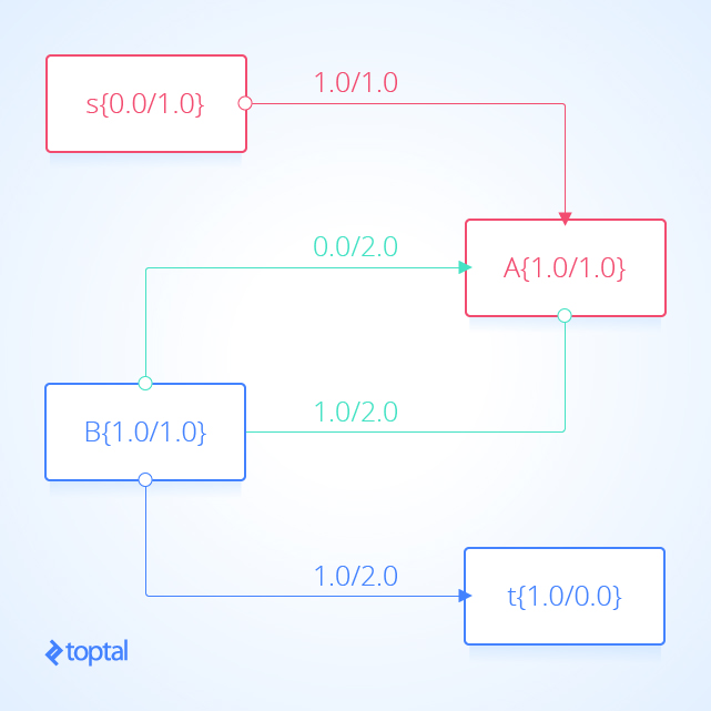
Corollary: No s-t cut flow value can exceed the capacity of any s-t cut .
Proposition F. (max flow, min cut theorem): Let f be an s-t flow . The following 3 conditions are equivalent:
There exists an s-t cut whose capacity equals the value of the flow f .
f is a max flow .
There is no augmenting path with respect to f .
Condition 1 implies condition 2 by the corollary. Condition 2 implies condition 3 because the existence of an augmenting path implies the existence of a flow with larger values, contradicting the maximality of f . Condition 3 implies condition 1: Let C_s be the set of all nodes that can be reached from s with an augmenting path in the residual graph . Let C_t be the remaining arcs , then t must be in C_t (by our assumption). The arcs crossing from C_s to C_t then form an s-t cut which contains only arcs a where either a.datum.capacity = a.datum.flow or a.datum.flow = 0.0 . If this were otherwise then the nodes connected by an arc with remaining residual capacity to C_s would be in the set C_s since there would then be an augmenting path from s to such a node . The flow across the s-t cut is equal to the s-t cut’s capacity (since arcs from C_s to C_t have flow equal to capacity) and also to the value of the s-t flow (by proposition E ).
This statement of the max flow, min cut theorem implies the earlier statement from Flows in Networks .
Corollary (integrality property): When capacities are integers, there exists an integer-valued max flow, and the Ford-Fulkerson algorithm finds it.
Proof: Each augmenting path increases the flow by a positive integer, the minimum of the unused capacities in the ‘push’ arcs and the flows in the ‘pull’ arcs , all of which are always positive integers.
This justifies the Ford-Fulkerson method description from CLRS . The method is to keep finding augmenting paths and applying augment to the latest maxFlowSolution coming up with better solutions, until no more augmenting path meaning that the latest maximum flow solution is optimal .
From Ford-Fulkerson to Edmonds-Karp
The remaining questions regarding solving maximum flow problems are:
How should augmenting paths be constructed?
Will the method terminate if we use real numbers and not integers?
How long will it take to terminate (if it does)?
The Edmonds-Karp algorithm specifies that each augmenting path is constructed by a breadth first search ( BFS ) of the residual graph ; it turns out that this decision of point 1 above will also force the algorithm to terminate (point 2) and allows the asymptotic time and space complexity to be determined.
First, here’s a BFS implementation:
I used a deque from the python collections module .
To answer question 2 above, I’ll paraphrase another proof from Sedgewick and Wayne : Proposition G. The number of augmenting paths needed in the Edmonds-Karp algorithm with N nodes and A arcs is at most NA/2 . Proof: Every augmenting path has a bottleneck arc - an arc that is deleted from the residual graph because it corresponds either to a ‘push’ arc that becomes filled to capacity or a ‘pull’ arc through which the flow becomes 0. Each time an arc becomes a bottleneck arc , the length of any augmenting path through it must increase by a factor of 2. This is because each node in a path may appear only once or not at all (from the definition of path ) since the paths are being explored from shortest path to longest that means that at least one more node must be visited by the next path that goes through the particular bottleneck node that means an additional 2 arcs on the path before we arrive at the node . Since the augmenting path is of length at most N each arc can be on at most N/2 augmenting paths , and the total number of augmenting paths is at most NA/2 .
The Edmonds-Karp algorithm executes in O(NA^2) . If at most NA/2 paths will be explored during the algorithm and exploring each path with BFS is N+A then the most significant term of the product and hence the asymptotic complexity is O(NA^2) .
Let mfp be a maxFlowProblemState .
The version above is inefficient and has worse complexity than O(NA^2) since it constructs a new maximum flow solution and new a residual graph each time (rather than modifying existing digraphs as the algorithm advances). To get to a true O(NA^2) solution the algorithm must maintain both the digraph representing the maximum flow problem state and its associated residual graph . So the algorithm must avoid iterating over arcs and nodes unnecessarily and update their values and associated values in the residual graph only as necessary.
To write a faster Edmonds Karp algorithm, I rewrote several pieces of code from the above. I hope that going through the code which generated a new digraph was helpful in understanding what’s going on. In the fast algorithm, I use some new tricks and Python data structures that I don’t want to go over in detail. I will say that a.fromNode and a.toNode are now treated as strings and uids to nodes . For this code, let mfps be a maxFlowProblemState
Here’s a visualization of how this algorithm solves the example flow network from above. The visualization shows the steps as they are reflected in the digraph G representing the most up-to-date flow network and as they are reflected in the residual graph of that flow network. Augmenting paths in the residual graph are shown as red paths, and the digraph representing the problem the set of nodes and arcs affected by a given augmenting path is highlighted in green. In each case, I’ll highlight the parts of the graph that will be changed (in red or green) and then show the graph after the changes (just in black).
Here’s another visualization of how this algorithm solving a different example flow network . Notice that this one uses real numbers and contains multiple arcs with the same fromNode and toNode values.
**Also notice that because Arcs with a ‘pull’ ResidualDatum may be part of the Augmenting Path, the nodes affected in the DiGraph of the Flown Network _may not be on a path in G! .
Bipartite Graphs
Suppose we have a digraph G , G is bipartite if it’s possible to partition the nodes in G.setOfNodes into two sets ( part_1 and part_2 ) such that for any arc a in G.setOfArcs it cannot be true that a.fromNode in part_1 and a.toNode in part_1 . It also cannot be true that a.fromNode in part_2 and a.toNode in part_2 .
In other words G is bipartite if it can be partitioned into two sets of nodes such that every arc must connect a node in one set to a node in the other set.
Testing Bipartite
Suppose we have a digraph G , we want to test if it is bipartite . We can do this in O(|G.setOfNodes|+|G.setOfArcs|) by greedy coloring the graph into two colors.
First, we need to generate a new digraph H . This graph will have will have the same set of nodes as G , but it will have more arcs than G . Every arc a in G will create 2 arcs in H ; the first arc will be identical to a , and the second arc reverses the director of a ( b = Arc(a.toNode,a.fromNode,a.datum) ).
Matchings and Maximum Matchings
Suppose we have a digraph G and matching is a subset of arcs from G.setOfArcs . matching is a matching if for any two arcs a and b in matching : len(frozenset( {a.fromNode} ).union( {a.toNode} ).union( {b.fromNode} ).union( {b.toNode} )) == 4 . In other words, no two arcs in a matching share a node .
Matching matching , is a maximum matching if there is no other matching alt_matching in G such that len(matching) < len(alt_matching) . In other words, matching is a maximum matching if it is the largest set of arcs from G.setOfArcs that still satisfies the definition of matching (the addition of any arc not already in the matching will break the matching definition).
A maximum matching matching is a perfect matching if every for node n in G.setOfArcs there exists an arc a in matching where a.fromNode == n or a.toNode == n .
Maximum Bipartite Matching
A maximum bipartite matching is a maximum matching on a digraph G which is bipartite .
Given that G is bipartite , the problem of finding a maximum bipartite matching can be transformed into a maximum flow problem solvable with the Edmonds-Karp algorithm and then the maximum bipartite matching can be recovered from the solution to the maximum flow problem .
Let bipartition be a bipartition of G .
To do this, I need to generate a new digraph ( H ) with some new nodes ( H.setOfNodes ) and some new arcs ( H.setOfArcs ). H.setOfNodes contains all the nodes in G.setOfNodes and two more nodess , s (a source node ) and t (a terminal node ).
H.setOfArcs will contain one arc for each G.setOfArcs . If an arc a is in G.setOfArcs and a.fromNode is in bipartition.firstPart and a.toNode is in bipartition.secondPart then include a in H (adding a FlowArcDatum(1,0) ).
If a.fromNode is in bipartition.secondPart and a.toNode is in bipartition.firstPart , then include Arc(a.toNode,a.fromNode,FlowArcDatum(1,0)) in H.setOfArcs .
The definition of a bipartite graph ensures that no arc connects any nodes where both nodes are in the same partition. H.setOfArcs also contains an arc from node s to each node in bipartition.firstPart . Finally, H.setOfArcs contains an arc each node in bipartition.secondPart to node t . a.datum.capacity = 1 for all a in H.setOfArcs .
First partition the nodes in G.setOfNodes the two disjoint sets ( part1 and part2 ) such that no arc in G.setOfArcs is directed from one set to the same set (this partition is possible because G is bipartite ). Next, add all arcs in G.setOfArcs which are directed from part1 to part2 into H.setOfArcs . Then create a single source node s and a single terminal node t and create some more arcs
Then, construct a maxFlowProblemState .
Minimal Node Cover
A node cover in a digraph G is a set of nodes ( cover ) from G.setOfNodes such that for any arc a of G.setOfArcs this must be true: (a.fromNode in cover) or (a.toNode in cover) .
A minimal node cover is the smallest possible set of nodes in the graph that is still a node cover . König’s theorem states that in a bipartite graph, the size of the maximum matching on that graph is equal to the size of the minimal node cover , and it suggests how the node cover can recovered from a maximum matching :
Suppose we have the bipartition bipartition and the maximum matching matching . Define a new digraph H , H.setOfNodes=G.setOfNodes , the arcs in H.setOfArcs are the union of two sets.
The first set is arcs a in matching , with the change that if a.fromNode in bipartition.firstPart and a.toNode in bipartition.secondPart then a.fromNode and a.toNode are swapped in the created arc give such arcs a a.datum.inMatching=True attribute to indicate that they were derived from arcs in a matching .
The second set is arcs a NOT in matching , with the change that if a.fromNode in bipartition.secondPart and a.toNode in bipartition.firstPart then a.fromNode and a.toNode are swapped in the created arc (give such arcs a a.datum.inMatching=False attribute).
Next, run a depth first search ( DFS ) starting from each node n in bipartition.firstPart which is neither n == a.fromNode nor n == a.toNodes for any arc a in matching . During the DFS, some nodes are visited and some are not (store this information in a n.datum.visited field). The minimum node cover is the union of the nodes {a.fromNode for a in H.setOfArcs if ( (a.datum.inMatching) and (a.fromNode.datum.visited) ) } and the nodes {a.fromNode for a in H.setOfArcs if (a.datum.inMatching) and (not a.toNode.datum.visited)} .
This can be shown to lead from a maximum matching to a minimal node cover by a proof by contradiction , take some arc a that was supposedly not covered and consider all four cases regarding whether a.fromNode and a.toNode belong (whether as toNode or fromNode ) to any arc in matching matching . Each case leads to a contradiction due to the order that DFS visits nodes and the fact that matching is a maximum matching .
Suppose we have a function to execute these steps and return the set of nodes comprising the minimal node cover when given the digraph G , and the maximum matching matching :
The Linear Assignment Problem
The linear assignment problem consists of finding a maximum weight matching in a weighted bipartite graph.
Problems like the one at the very start of this post can be expressed as a linear assignment problem . Given a set of workers, a set of tasks, and a function indicating the profitability of an assignment of one worker to one task, we want to maximize the sum of all assignments that we make; this is a linear assignment problem .
Assume that the number of tasks and workers are equal, though I will show that this assumption is easy to remove. In the implementation, I represent arc weights with an attribute a.datum.weight for an arc a .
Kuhn-Munkres Algorithm
The Kuhn-Munkres Algorithm solves the linear assignment problem . A good implementation can take O(N^{4}) time, (where N is the number of nodes in the digraph representing the problem). An implementation that is easier to explain takes O(N^{5}) (for a version which regenerates DiGraphs ) and O(N^{4}) for (for a version which maintains DiGraphs ). This is similar to the two different implementations of the Edmonds-Karp algorithm.
For this description, I’m only working with complete bipartite graphs (those where half the nodes are in one part of the bipartition and the other half in the second part). In the worker, task motivation this means that there are as many workers as tasks.
This seems like a significant condition (what if these sets are not equal!) but it is easy to fix this issue; I talk about how to do that in the last section.
The version of the algorithm described here uses the useful concept of zero weight arcs . Unfortunately, this concept only makes sense when we are solving a minimization (if rather than maximizing the profits of our worker-task assignments we were instead minimizing the cost of such assignments).
Fortunately, it is easy to turn a maximum linear assignment problem into a minimum linear assignment problem by setting each the arc a weights to M-a.datum.weight where M=max({a.datum.weight for a in G.setOfArcs}) . The solution to the original maximizing problem will be identical to the solution minimizing problem after the arc weights are changed. So for the remainder, assume that we make this change.
The Kuhn-Munkres algorithm solves minimum weight matching in a weighted bipartite graph by a sequence of maximum matchings in unweighted bipartite graphs. If a we find a perfect matching on the digraph representation of the linear assignment problem , and if the weight of every arc in the matching is zero, then we have found the minimum weight matching since this matching suggests that all nodes in the digraph have been matched by an arc with the lowest possible cost (no cost can be lower than 0, based on prior definitions).
No other arcs can be added to the matching (because all nodes are already matched) and no arcs should be removed from the matching because any possible replacement arc will have at least as great a weight value.
If we find a maximum matching of the subgraph of G which contains only zero weight arcs , and it is not a perfect matching , we don’t have a full solution (since the matching is not perfect ). However, we can produce a new digraph H by changing the weights of arcs in G.setOfArcs in a way that new 0-weight arcs appear and the optimal solution of H is the same as the optimal solution of G . Since we guarantee that at least one zero weight arc is produced at each iteration, we guarantee that we will arrive at a perfect matching in no more than |G.setOfNodes|^{2}=N^{2} such iterations.
Suppose that in bipartition bipartition , bipartition.firstPart contains nodes representing workers, and bipartition.secondPart represents nodes representing tasks.
The algorithm starts by generating a new digraph H . H.setOfNodes = G.setOfNodes . Some arcs in H are generated from nodes n in bipartition.firstPart . Each such node n generates an arc b in H.setOfArcs for each arc a in bipartition.G.setOfArcs where a.fromNode = n or a.toNode = n , b=Arc(a.fromNode, a.toNode, a.datum.weight - z) where z=min(x.datum.weight for x in G.setOfArcs if ( (x.fromNode == n) or (x.toNode == n) )) .
More arcs in H are generated from nodes n in bipartition.secondPart . Each such node n generates an arc b in H.setOfArcs for each arc a in bipartition.G.setOfArcs where a.fromNode = n or a.toNode = n , b=Arc(a.fromNode, a.toNode, ArcWeightDatum(a.datum.weight - z)) where z=min(x.datum.weight for x in G.setOfArcs if ( (x.fromNode == n) or (x.toNode == n) )) .
KMA: Next, form a new digraph K composed of only the zero weight arcs from H , and the nodes incident on those arcs . Form a bipartition on the nodes in K , then use solve_mbm( bipartition ) to get a maximum matching ( matching ) on K . If matching is a perfect matching in H (the arcs in matching are incident on all nodes in H.setOfNodes ) then the matching is an optimal solution to the linear assignment problem .
Otherwise, if matching is not perfect , generate the minimal node cover of K using node_cover = get_min_node_cover(matching, bipartition(K)) . Next, define z=min({a.datum.weight for a in H.setOfArcs if a not in node_cover}) . Define nodes = H.setOfNodes , arcs1 = {Arc(a.fromNode,a.toNode,ArcWeightDatum(a.datum.weigh-z)) for a in H.setOfArcs if ( (a.fromNode not in node_cover) and (a.toNode not in node_cover)} , arcs2 = {Arc(a.fromNode,a.toNode,ArcWeightDatum(a.datum.weigh)) for a in H.setOfArcs if ( (a.fromNode not in node_cover) != (a.toNode not in node_cover)} , arcs3 = {Arc(a.fromNode,a.toNode,ArcWeightDatum(a.datum.weigh+z)) for a in H.setOfArcs if ( (a.fromNode in node_cover) and (a.toNode in node_cover)} . The != symbol in the previous expression acts as an XOR operator. Then arcs = arcs1.union(arcs2.union(arcs3)) . Next, H=DiGraph(nodes,arcs) . Go back to the label KMA . The algorithm continues until a perfect matching is produced. This matching is also the solution to the linear assignment problem .
This implementation is O(N^{5}) because it generates a new maximum matching matching at each iteration; similar to the previous two implementations of Edmonds-Karp this algorithm can be modified so that it keeps track of the matching and adapts it intelligently to each iteration. When this is done, the complexity becomes O(N^{4}) . A more advanced and more recent version of this algorithm (requiring some more advanced data structures) can run in O(N^{3}) . Details of both the simpler implementation above and the more advanced implementation can be found at this post which motivated this blog post.
None of the operations on arc weights modify the final assignment returned by the algorithm. Here’s why: Since our input graphs are always complete bipartite graphs a solution must map each node in one partition to another node in the second partition, via the arc between these two nodes . Notice that the operations performed on the arc weights never changes the order (ordered by weight) of the arcs incident on any particular node .
Thus when the algorithm terminates at a perfect complete bipartite matching each node is assigned a zero weight arc , since the relative order of the arcs from that node hasn’t changed during the algorithm, and since a zero weight arc is the cheapest possible arc and the perfect complete bipartite matching guarantees that one such arc exists for each node . This means that the solution generated is indeed the same as the solution from the original linear assignment problem without any modification of arc weights.
Unbalanced Assignments
It seems like the algorithm is quite limited since as described it operates only on complete bipartite graphs (those where half the nodes are in one part of the bipartition and the other half in the second part). In the worker, task motivation this means that there are as many workers as tasks (seems quite limiting).
However, there is an easy transformation that removes this restriction. Suppose that there are fewer workers than tasks, we add some dummy workers (enough to make the resulting graph a complete bipartite graph ). Each dummy worker has an arc directed from the worker to each of the tasks. Each such arc has weight 0 (placing it in a matching gives no added profit). After this change the graph is a complete bipartite graph which we can solve for. Any task assigned a dummy worker is not initiated.
Suppose that there are more tasks than workers. We add some dummy tasks (enough to make the resulting graph a complete bipartite graph ). Each dummy task has an arc directed from each worker to the dummy task. Each such arc has a weight of 0 (placing it in a matching gives no added profit). After this change the graph is a complete bipartite graph which we can solve for. Any worker assigned to dummy task is not employed during the period.
A Linear Assignment Example
Finally, let’s do an example with the code I’ve been using. I’m going to modify the example problem from here . We have 3 tasks: we need to clean the bathroom , sweep the floor , and wash the windows .
The workers available to use are Alice , Bob , Charlie , and Diane . Each of the workers gives us the wage they require per task. Here are the wages per worker:
| Clean the Bathroom | Sweep the Floor | Wash the Windows | |
|---|---|---|---|
| Alice | $2 | $3 | $3 |
| Bob | $3 | $2 | $3 |
| Charlie | $3 | $3 | $2 |
| Diane | $9 | $9 | $1 |
If we want to pay the least amount of money, but still get all the tasks done, who should do what task? Start by introducing a dummy task to make the digraph representing the problem bipartite.
| Clean the Bathroom | Sweep the Floor | Wash the Windows | Do Nothing | |
|---|---|---|---|---|
| Alice | $2 | $3 | $3 | $0 |
| Bob | $3 | $2 | $3 | $0 |
| Charlie | $3 | $3 | $2 | $0 |
| Diane | $9 | $9 | $1 | $0 |
Supposing that the problem is encoded in a digraph , then kuhn_munkres( bipartition(G) ) will solve the problem and return the assignment. It’s easy to verify that the optimal (lowest cost) assignment will cost $5.
Here’s a visualization of the solution the code above generates:
That is it. You now know everything you need to know about the linear assignment problem.
You can find all of the code from this article on GitHub .
Further Reading on the Toptal Blog:
- Graph Data Science With Python/NetworkX
Dmitri Ivanovich Arkhipov
Irvine, CA, United States
Member since January 23, 2017
About the author
World-class articles, delivered weekly.
By entering your email, you are agreeing to our privacy policy .
Toptal Developers
- Adobe Commerce (Magento) Developers
- Angular Developers
- AWS Developers
- Azure Developers
- Big Data Architects
- Blockchain Developers
- Business Intelligence Developers
- C Developers
- Computer Vision Developers
- Django Developers
- Docker Developers
- Elixir Developers
- Go Engineers
- GraphQL Developers
- Jenkins Developers
- Kotlin Developers
- Kubernetes Developers
- .NET Developers
- R Developers
- React Native Developers
- Ruby on Rails Developers
- Salesforce Developers
- Tableau Developers
- Unreal Engine Developers
- Xamarin Developers
- View More Freelance Developers
Join the Toptal ® community.
Navigation Menu
Search code, repositories, users, issues, pull requests..., provide feedback.
We read every piece of feedback, and take your input very seriously.
Saved searches
Use saved searches to filter your results more quickly.
To see all available qualifiers, see our documentation .
linear-assignment-problem
Here are 6 public repositories matching this topic..., kcg2015 / vehicle-detection-and-tracking.
Computer vision based vehicle detection and tracking using Tensorflow Object Detection API and Kalman-filtering
- Updated May 23, 2020
cheind / py-lapsolver
Fast linear assignment problem (LAP) solvers for Python based on c-extensions
- Updated Dec 22, 2023
bkj / auction-lap
Auction algorithm for solving linear assignment problem (LAP)
- Updated Jun 21, 2022
yfukai / laptrack
Particle tracking by solving linear assignment problem.
- Updated Aug 5, 2024
OllieBoyne / sslap
Auction Algorithm for Sparse Linear Assignment Problems
- Updated Mar 15, 2021
berhane / arbalign
aligns arbitrarily ordered isomers
- Updated Dec 28, 2019
Improve this page
Add a description, image, and links to the linear-assignment-problem topic page so that developers can more easily learn about it.
Curate this topic
Add this topic to your repo
To associate your repository with the linear-assignment-problem topic, visit your repo's landing page and select "manage topics."
- Stack Overflow for Teams Where developers & technologists share private knowledge with coworkers
- Advertising & Talent Reach devs & technologists worldwide about your product, service or employer brand
- OverflowAI GenAI features for Teams
- OverflowAPI Train & fine-tune LLMs
- Labs The future of collective knowledge sharing
- About the company Visit the blog
Collectives™ on Stack Overflow
Find centralized, trusted content and collaborate around the technologies you use most.
Q&A for work
Connect and share knowledge within a single location that is structured and easy to search.
Get early access and see previews of new features.
How do I resolve "Use scipy.optimize.linear_sum_assignment instead"
I am using python script for people detection. I have the following line in my script:
When I run my script I have got the following lines:
Please, advice me how to solve it.
2 Answers 2
You need to replace the sklearn.utils.linear_assignment_.linear_assignment function by the scipy.optimize.linear_sum_assignment function .
The difference is in the return format: linear_assignment() is returning a numpy array and linear_sum_assignment() a tuple of numpy arrays . You obtain the same output by converting the output of linear_sum_assignment() in array and transpose it.
Your script should look like this:
Replace the linear_assignment for linear_sum_assignment
https://docs.scipy.org/doc/scipy/reference/generated/scipy.optimize.linear_sum_assignment.html
Your Answer
Reminder: Answers generated by artificial intelligence tools are not allowed on Stack Overflow. Learn more
Sign up or log in
Post as a guest.
Required, but never shown
By clicking “Post Your Answer”, you agree to our terms of service and acknowledge you have read our privacy policy .
Not the answer you're looking for? Browse other questions tagged python or ask your own question .
- The Overflow Blog
- Where does Postgres fit in a world of GenAI and vector databases?
- Featured on Meta
- We've made changes to our Terms of Service & Privacy Policy - July 2024
- Bringing clarity to status tag usage on meta sites
- What does a new user need in a homepage experience on Stack Overflow?
- Feedback requested: How do you use tag hover descriptions for curating and do...
- Staging Ground Reviewer Motivation
Hot Network Questions
- I'm trying to remember a novel about an asteroid threatening to destroy the earth. I remember seeing the phrase "SHIVA IS COMING" on the cover
- Integral concerning the floor function
- Why is PUT Request not allowed by default in OWASP CoreRuleSet
- How can these humans cross the ocean(s) at the first possible chance?
- "TSA regulations state that travellers are allowed one personal item and one carry on"?
- How much missing data is too much (part 2)? statistical power, effective sample size
- A way to move an object with the 3D cursor location as the moving point?
- Parse Minecraft's VarInt
- Relation between stopping times and their filtrations
- Which programming language/environment pioneered row-major array order?
- Purpose of burn permit?
- Is Intuition Indispensable in Mathematics?
- What happens if all nine Supreme Justices recuse themselves?
- How to reply to reviewers who ask for more work by responding that the paper is complete as it stands?
- Historical U.S. political party "realignments"?
- Slicing Graph by path
- What is the difference between a "Complaint for Civil Protection Order" and a "Motion for Civil Protection Order"?
- Distinctive form of "לאהוב ל-" instead of "לאהוב את"
- Expected number of numbers that stay at their place after k swaps
- Safety pictograms
- A very interesting food chain
- How can I delete a column from several CSV files?
- The size of elementary particles
- Parody of Fables About Authenticity
scipy.optimize.linear_sum_assignment #
Solve the linear sum assignment problem.
The cost matrix of the bipartite graph.
Calculates a maximum weight matching if true.
An array of row indices and one of corresponding column indices giving the optimal assignment. The cost of the assignment can be computed as cost_matrix[row_ind, col_ind].sum() . The row indices will be sorted; in the case of a square cost matrix they will be equal to numpy.arange(cost_matrix.shape[0]) .
for sparse inputs
The linear sum assignment problem [1] is also known as minimum weight matching in bipartite graphs. A problem instance is described by a matrix C, where each C[i,j] is the cost of matching vertex i of the first partite set (a ‘worker’) and vertex j of the second set (a ‘job’). The goal is to find a complete assignment of workers to jobs of minimal cost.
Formally, let X be a boolean matrix where \(X[i,j] = 1\) iff row i is assigned to column j. Then the optimal assignment has cost
where, in the case where the matrix X is square, each row is assigned to exactly one column, and each column to exactly one row.
This function can also solve a generalization of the classic assignment problem where the cost matrix is rectangular. If it has more rows than columns, then not every row needs to be assigned to a column, and vice versa.
This implementation is a modified Jonker-Volgenant algorithm with no initialization, described in ref. [2] .
New in version 0.17.0.
https://en.wikipedia.org/wiki/Assignment_problem
DF Crouse. On implementing 2D rectangular assignment algorithms. IEEE Transactions on Aerospace and Electronic Systems , 52(4):1679-1696, August 2016, DOI:10.1109/TAES.2016.140952
IMAGES
VIDEO
COMMENTS
The linear sum assignment problem [1] is also known as minimum weight matching in bipartite graphs. A problem instance is described by a matrix C, where each C [i,j] is the cost of matching vertex i of the first partite set (a 'worker') and vertex j of the second set (a 'job'). The goal is to find a complete assignment of workers to ...
In this step, we will solve the LP problem by calling solve () method. We can print the final value by using the following for loop. From the above results, we can infer that Worker-1 will be assigned to Job-1, Worker-2 will be assigned to job-3, Worker-3 will be assigned to Job-2, and Worker-4 will assign with job-4.
The linear sum assignment problem is also known as minimum weight matching in bipartite graphs. A problem instance is described by a matrix C, where each C [i,j] is the cost of matching vertex i of the first partite set (a "worker") and vertex j of the second set (a "job"). The goal is to find a complete assignment of workers to jobs of ...
The program uses the linear assignment solver, a specialized solver for the assignment problem. The following code creates the solver. Note: The linear sum assignment solver only accepts integer values for the weights and values. The section Using a solver with non-integer data shows how to use the solver if your data contains non-integer values.
py-lapsolver implements a Linear sum Assignment Problem (LAP) solver for dense matrices based on shortest path augmentation in Python. In practice, it solves 5000x5000 problems in around 3 seconds. In practice, it solves 5000x5000 problems in around 3 seconds.
Linear Assignment Problem solver using Jonker-Volgenant algorithm. This project is the rewrite of pyLAPJV which supports Python 3 and updates the core code. The performance is twice as high as the original thanks to the optimization of the augmenting row reduction phase using Intel AVX2 intrinsics. It is a native Python 3 module and does not ...
The linear assignment problem (or simply assignment problem) is the problem of finding a matching between two sets that minimizes the sum of pair-wise assignment costs. ... Python packages. The table below outlines the different behaviour of several popular packages.
The problem is to assign each worker to at most one task, with no two workers performing the same task, while minimizing the total cost. Since there are more workers than tasks, one worker will not be assigned a task. MIP solution. The following sections describe how to solve the problem using the MPSolver wrapper. Import the libraries
lapx basically is Tomas Kazmar's gatagat/lap with support for all Windows/Linux/macOS and Python 3.7-3.12.. About lap. Tomas Kazmar's lap is a linear assignment problem solver using Jonker-Volgenant algorithm for dense LAPJV ¹ or sparse LAPMOD ² matrices. Both algorithms are implemented from scratch based solely on the papers ¹˒² and the public domain Pascal implementation provided by A ...
6. No, NumPy contains no such function. Combinatorial optimization is outside of NumPy's scope. It may be possible to do it with one of the optimizers in scipy.optimize but I have a feeling that the constraints may not be of the right form. NetworkX probably also includes algorithms for assignment problems.
Purpose. The script benchmarks the performance of Python3 linear assignment problem solvers for random cost matrices of different sizes. These solvers are: lapjv.lapjv - a wrapper to a C++ implementation of Jonker-Volgenant algorithm re-written for Python 3 and optimized to take advantage of AVX2 instruction sets by Vadim Markovtsev at src {d}.
The linear sum assignment problem [1] is also known as minimum weight matching in bipartite graphs. A problem instance is described by a matrix C, where each C [i,j] is the cost of matching vertex i of the first partite set (a 'worker') and vertex j of the second set (a 'job'). The goal is to find a complete assignment of workers to ...
You'll use Python to solve these two problems in the next section. Small Linear Programming Problem. Consider the following linear programming problem: You need to find x and y such that the red, blue, and yellow inequalities, as well as the inequalities x ≥ 0 and y ≥ 0, are satisfied.
Linear Assignment problems are fundamental combinatorial optimization problems. In most general form, the problem instance has a number of agents and a number of tasks. ... Python Libraries for ...
lap is a linear assignment problem solver using Jonker-Volgenant algorithm for dense (LAPJV [1]) or sparse (LAPMOD [2]) matrices.. Both algorithms are implemented from scratch based solely on the papers [1,2] and the public domain Pascal implementation provided by A. Volgenant [3].
Fortunately, it is easy to turn a maximum linear assignment problem into a minimum linear assignment problem by setting each the arc a weights to M-a.datum.weight where M=max({a.datum.weight for a in G.setOfArcs}). The solution to the original maximizing problem will be identical to the solution minimizing problem after the arc weights are ...
The linear sum assignment problem [1] is also known as minimum weight matching in bipartite graphs. A problem instance is described by a matrix C, where each C [i,j] is the cost of matching vertex i of the first partite set (a 'worker') and vertex j of the second set (a 'job'). The goal is to find a complete assignment of workers to ...
The linear sum assignment problem is also known as minimum weight matching in bipartite graphs. A problem instance is described by a matrix C, where each C [i,j] is the cost of matching vertex i of the first partite set (a "worker") and vertex j of the second set (a "job"). The goal is to find a complete assignment of workers to jobs of ...
Add this topic to your repo. To associate your repository with the linear-assignment-problem topic, visit your repo's landing page and select "manage topics." GitHub is where people build software. More than 100 million people use GitHub to discover, fork, and contribute to over 420 million projects.
22. You need to replace the sklearn.utils.linear_assignment_.linear_assignment function by the scipy.optimize.linear_sum_assignment function. The difference is in the return format: linear_assignment() is returning a numpy array and linear_sum_assignment() a tuple of numpy arrays. You obtain the same output by converting the output of linear ...
The linear sum assignment problem [1] is also known as minimum weight matching in bipartite graphs. A problem instance is described by a matrix C, where each C [i,j] is the cost of matching vertex i of the first partite set (a 'worker') and vertex j of the second set (a 'job'). The goal is to find a complete assignment of workers to ...