writing correlation hypothesis

User Preferences

Content preview.

Arcu felis bibendum ut tristique et egestas quis:

• Ut enim ad minim veniam, quis nostrud exercitation ullamco laboris
• Duis aute irure dolor in reprehenderit in voluptate
• Excepteur sint occaecat cupidatat non proident

Keyboard Shortcuts

5.2 - writing hypotheses.

The first step in conducting a hypothesis test is to write the hypothesis statements that are going to be tested. For each test you will have a null hypothesis (\(H_0\)) and an alternative hypothesis (\(H_a\)).

When writing hypotheses there are three things that we need to know: (1) the parameter that we are testing (2) the direction of the test (non-directional, right-tailed or left-tailed), and (3) the value of the hypothesized parameter.

• At this point we can write hypotheses for a single mean (\(\mu\)), paired means(\(\mu_d\)), a single proportion (\(p\)), the difference between two independent means (\(\mu_1-\mu_2\)), the difference between two proportions (\(p_1-p_2\)), a simple linear regression slope (\(\beta\)), and a correlation (\(\rho\)). 
• The research question will give us the information necessary to determine if the test is two-tailed (e.g., "different from," "not equal to"), right-tailed (e.g., "greater than," "more than"), or left-tailed (e.g., "less than," "fewer than").
• The research question will also give us the hypothesized parameter value. This is the number that goes in the hypothesis statements (i.e., \(\mu_0\) and \(p_0\)). For the difference between two groups, regression, and correlation, this value is typically 0.

Hypotheses are always written in terms of population parameters (e.g., \(p\) and \(\mu\)).  The tables below display all of the possible hypotheses for the parameters that we have learned thus far. Note that the null hypothesis always includes the equality (i.e., =).

12.4 Testing the Significance of the Correlation Coefficient

The correlation coefficient, r , tells us about the strength and direction of the linear relationship between x and y . However, the reliability of the linear model also depends on how many observed data points are in the sample. We need to look at both the value of the correlation coefficient r and the sample size n , together.

We perform a hypothesis test of the "significance of the correlation coefficient" to decide whether the linear relationship in the sample data is strong enough to use to model the relationship in the population.

The sample data are used to compute r , the correlation coefficient for the sample. If we had data for the entire population, we could find the population correlation coefficient. But because we have only sample data, we cannot calculate the population correlation coefficient. The sample correlation coefficient, r , is our estimate of the unknown population correlation coefficient.

• The symbol for the population correlation coefficient is ρ , the Greek letter "rho."
• ρ = population correlation coefficient (unknown)
• r = sample correlation coefficient (known; calculated from sample data)

The hypothesis test lets us decide whether the value of the population correlation coefficient ρ is "close to zero" or "significantly different from zero". We decide this based on the sample correlation coefficient r and the sample size n .

If the test concludes that the correlation coefficient is significantly different from zero, we say that the correlation coefficient is "significant."

• Conclusion: There is sufficient evidence to conclude that there is a significant linear relationship between x and y because the correlation coefficient is significantly different from zero.
• What the conclusion means: There is a significant linear relationship between x and y . We can use the regression line to model the linear relationship between x and y in the population.

If the test concludes that the correlation coefficient is not significantly different from zero (it is close to zero), we say that correlation coefficient is "not significant".

• Conclusion: "There is insufficient evidence to conclude that there is a significant linear relationship between x and y because the correlation coefficient is not significantly different from zero."
• What the conclusion means: There is not a significant linear relationship between x and y . Therefore, we CANNOT use the regression line to model a linear relationship between x and y in the population.
• If r is significant and the scatter plot shows a linear trend, the line can be used to predict the value of y for values of x that are within the domain of observed x values.
• If r is not significant OR if the scatter plot does not show a linear trend, the line should not be used for prediction.
• If r is significant and if the scatter plot shows a linear trend, the line may NOT be appropriate or reliable for prediction OUTSIDE the domain of observed x values in the data.

PERFORMING THE HYPOTHESIS TEST

• Null Hypothesis: H 0 : ρ = 0
• Alternate Hypothesis: H a : ρ ≠ 0

WHAT THE HYPOTHESES MEAN IN WORDS:

• Null Hypothesis H 0 : The population correlation coefficient IS NOT significantly different from zero. There IS NOT a significant linear relationship (correlation) between x and y in the population.
• Alternate Hypothesis H a : The population correlation coefficient IS significantly DIFFERENT FROM zero. There IS A SIGNIFICANT LINEAR RELATIONSHIP (correlation) between x and y in the population.

DRAWING A CONCLUSION: There are two methods of making the decision. The two methods are equivalent and give the same result.

• Method 1: Using the p -value
• Method 2: Using a table of critical values

In this chapter of this textbook, we will always use a significance level of 5%, α = 0.05

Using the p -value method, you could choose any appropriate significance level you want; you are not limited to using α = 0.05. But the table of critical values provided in this textbook assumes that we are using a significance level of 5%, α = 0.05. (If we wanted to use a different significance level than 5% with the critical value method, we would need different tables of critical values that are not provided in this textbook.)

METHOD 1: Using a p -value to make a decision

Using the ti-83, 83+, 84, 84+ calculator.

To calculate the p -value using LinRegTTEST: On the LinRegTTEST input screen, on the line prompt for β or ρ , highlight " ≠ 0 " The output screen shows the p-value on the line that reads "p =". (Most computer statistical software can calculate the p -value.)

• Decision: Reject the null hypothesis.
• Conclusion: "There is sufficient evidence to conclude that there is a significant linear relationship between x and y because the correlation coefficient is significantly different from zero."
• Decision: DO NOT REJECT the null hypothesis.
• Conclusion: "There is insufficient evidence to conclude that there is a significant linear relationship between x and y because the correlation coefficient is NOT significantly different from zero."
• You will use technology to calculate the p -value. The following describes the calculations to compute the test statistics and the p -value:
• The p -value is calculated using a t -distribution with n - 2 degrees of freedom.
• The formula for the test statistic is t = r n − 2 1 − r 2 t = r n − 2 1 − r 2 . The value of the test statistic, t , is shown in the computer or calculator output along with the p -value. The test statistic t has the same sign as the correlation coefficient r .
• The p -value is the combined area in both tails.

An alternative way to calculate the p -value (p) given by LinRegTTest is the command 2*tcdf(abs(t),10^99, n-2) in 2nd DISTR.

• Consider the third exam/final exam example .
• The line of best fit is: ŷ = -173.51 + 4.83 x with r = 0.6631 and there are n = 11 data points.
• Can the regression line be used for prediction? Given a third exam score ( x value), can we use the line to predict the final exam score (predicted y value)?
• H 0 : ρ = 0
• H a : ρ ≠ 0
• The p -value is 0.026 (from LinRegTTest on your calculator or from computer software).
• The p -value, 0.026, is less than the significance level of α = 0.05.
• Decision: Reject the Null Hypothesis H 0
• Conclusion: There is sufficient evidence to conclude that there is a significant linear relationship between the third exam score ( x ) and the final exam score ( y ) because the correlation coefficient is significantly different from zero.

Because r is significant and the scatter plot shows a linear trend, the regression line can be used to predict final exam scores.

METHOD 2: Using a table of Critical Values to make a decision

The 95% Critical Values of the Sample Correlation Coefficient Table can be used to give you a good idea of whether the computed value of r r is significant or not . Compare r to the appropriate critical value in the table. If r is not between the positive and negative critical values, then the correlation coefficient is significant. If r is significant, then you may want to use the line for prediction.

Example 12.7

Suppose you computed r = 0.801 using n = 10 data points. df = n - 2 = 10 - 2 = 8. The critical values associated with df = 8 are -0.632 and + 0.632. If r < negative critical value or r > positive critical value, then r is significant. Since r = 0.801 and 0.801 > 0.632, r is significant and the line may be used for prediction. If you view this example on a number line, it will help you.

Try It 12.7

For a given line of best fit, you computed that r = 0.6501 using n = 12 data points and the critical value is 0.576. Can the line be used for prediction? Why or why not?

Example 12.8

Suppose you computed r = –0.624 with 14 data points. df = 14 – 2 = 12. The critical values are –0.532 and 0.532. Since –0.624 < –0.532, r is significant and the line can be used for prediction

Try It 12.8

For a given line of best fit, you compute that r = 0.5204 using n = 9 data points, and the critical value is 0.666. Can the line be used for prediction? Why or why not?

Example 12.9

Suppose you computed r = 0.776 and n = 6. df = 6 – 2 = 4. The critical values are –0.811 and 0.811. Since –0.811 < 0.776 < 0.811, r is not significant, and the line should not be used for prediction.

Try It 12.9

For a given line of best fit, you compute that r = –0.7204 using n = 8 data points, and the critical value is = 0.707. Can the line be used for prediction? Why or why not?

THIRD-EXAM vs FINAL-EXAM EXAMPLE: critical value method

Consider the third exam/final exam example . The line of best fit is: ŷ = –173.51+4.83 x with r = 0.6631 and there are n = 11 data points. Can the regression line be used for prediction? Given a third-exam score ( x value), can we use the line to predict the final exam score (predicted y value)?

• Use the "95% Critical Value" table for r with df = n – 2 = 11 – 2 = 9.
• The critical values are –0.602 and +0.602
• Since 0.6631 > 0.602, r is significant.
• Conclusion:There is sufficient evidence to conclude that there is a significant linear relationship between the third exam score ( x ) and the final exam score ( y ) because the correlation coefficient is significantly different from zero.

Example 12.10

Suppose you computed the following correlation coefficients. Using the table at the end of the chapter, determine if r is significant and the line of best fit associated with each r can be used to predict a y value. If it helps, draw a number line.

• r = –0.567 and the sample size, n , is 19. The df = n – 2 = 17. The critical value is –0.456. –0.567 < –0.456 so r is significant.
• r = 0.708 and the sample size, n , is nine. The df = n – 2 = 7. The critical value is 0.666. 0.708 > 0.666 so r is significant.
• r = 0.134 and the sample size, n , is 14. The df = 14 – 2 = 12. The critical value is 0.532. 0.134 is between –0.532 and 0.532 so r is not significant.
• r = 0 and the sample size, n , is five. No matter what the dfs are, r = 0 is between the two critical values so r is not significant.

Try It 12.10

For a given line of best fit, you compute that r = 0 using n = 100 data points. Can the line be used for prediction? Why or why not?

Assumptions in Testing the Significance of the Correlation Coefficient

Testing the significance of the correlation coefficient requires that certain assumptions about the data are satisfied. The premise of this test is that the data are a sample of observed points taken from a larger population. We have not examined the entire population because it is not possible or feasible to do so. We are examining the sample to draw a conclusion about whether the linear relationship that we see between x and y in the sample data provides strong enough evidence so that we can conclude that there is a linear relationship between x and y in the population.

The regression line equation that we calculate from the sample data gives the best-fit line for our particular sample. We want to use this best-fit line for the sample as an estimate of the best-fit line for the population. Examining the scatterplot and testing the significance of the correlation coefficient helps us determine if it is appropriate to do this.

• There is a linear relationship in the population that models the average value of y for varying values of x . In other words, the expected value of y for each particular value lies on a straight line in the population. (We do not know the equation for the line for the population. Our regression line from the sample is our best estimate of this line in the population.)
• The y values for any particular x value are normally distributed about the line. This implies that there are more y values scattered closer to the line than are scattered farther away. Assumption (1) implies that these normal distributions are centered on the line: the means of these normal distributions of y values lie on the line.
• The standard deviations of the population y values about the line are equal for each value of x . In other words, each of these normal distributions of y values has the same shape and spread about the line.
• The residual errors are mutually independent (no pattern).
• The data are produced from a well-designed, random sample or randomized experiment.

As an Amazon Associate we earn from qualifying purchases.

This book may not be used in the training of large language models or otherwise be ingested into large language models or generative AI offerings without OpenStax's permission.

Want to cite, share, or modify this book? This book uses the Creative Commons Attribution License and you must attribute OpenStax.

Access for free at https://openstax.org/books/introductory-statistics/pages/1-introduction

• Authors: Barbara Illowsky, Susan Dean
• Publisher/website: OpenStax
• Book title: Introductory Statistics
• Publication date: Sep 19, 2013
• Location: Houston, Texas
• Book URL: https://openstax.org/books/introductory-statistics/pages/1-introduction
• Section URL: https://openstax.org/books/introductory-statistics/pages/12-4-testing-the-significance-of-the-correlation-coefficient

© Jun 23, 2022 OpenStax. Textbook content produced by OpenStax is licensed under a Creative Commons Attribution License . The OpenStax name, OpenStax logo, OpenStax book covers, OpenStax CNX name, and OpenStax CNX logo are not subject to the Creative Commons license and may not be reproduced without the prior and express written consent of Rice University.

• Flashes Safe Seven
• FlashLine Login
• Faculty & Staff Phone Directory
• Emeriti or Retiree
• All Departments
• Maps & Directions

• Building Guide
• Departments
• Directions & Parking
• Faculty & Staff
• Give to University Libraries
• Library Instructional Spaces
• Mission & Vision
• Newsletters
• Circulation
• Course Reserves / Core Textbooks
• Equipment for Checkout
• Interlibrary Loan
• Library Instruction
• Library Tutorials
• My Library Account
• Open Access Kent State
• Research Support Services
• Statistical Consulting
• Student Multimedia Studio
• Citation Tools
• Databases A-to-Z
• Databases By Subject
• Digital Collections
• Discovery@Kent State
• Government Information
• Journal Finder
• Library Guides
• Connect from Off-Campus
• Library Workshops
• Subject Librarians Directory
• Suggestions/Feedback
• Writing Commons
• Academic Integrity
• Jobs for Students
• International Students
• Meet with a Librarian
• Study Spaces
• University Libraries Student Scholarship
• Affordable Course Materials
• Copyright Services
• Selection Manager
• Suggest a Purchase

Library Locations at the Kent Campus

• Architecture Library
• Fashion Library
• Map Library
• Performing Arts Library
• Special Collections and Archives

Regional Campus Libraries

• East Liverpool
• College of Podiatric Medicine

• Kent State University
• SPSS Tutorials

Pearson Correlation

Spss tutorials: pearson correlation.

• The SPSS Environment
• The Data View Window
• Using SPSS Syntax
• Data Creation in SPSS
• Importing Data into SPSS
• Variable Types
• Date-Time Variables in SPSS
• Defining Variables
• Creating a Codebook
• Computing Variables
• Computing Variables: Mean Centering
• Computing Variables: Recoding Categorical Variables
• Computing Variables: Recoding String Variables into Coded Categories (Automatic Recode)
• rank transform converts a set of data values by ordering them from smallest to largest, and then assigning a rank to each value. In SPSS, the Rank Cases procedure can be used to compute the rank transform of a variable." href="https://libguides.library.kent.edu/SPSS/RankCases" style="" >Computing Variables: Rank Transforms (Rank Cases)
• Weighting Cases
• Sorting Data
• Grouping Data
• Descriptive Stats for One Numeric Variable (Explore)
• Descriptive Stats for One Numeric Variable (Frequencies)
• Descriptive Stats for Many Numeric Variables (Descriptives)
• Descriptive Stats by Group (Compare Means)
• Frequency Tables
• Working with "Check All That Apply" Survey Data (Multiple Response Sets)
• Chi-Square Test of Independence
• One Sample t Test
• Paired Samples t Test
• Independent Samples t Test
• One-Way ANOVA
• How to Cite the Tutorials

Sample Data Files

Our tutorials reference a dataset called "sample" in many examples. If you'd like to download the sample dataset to work through the examples, choose one of the files below:

• Data definitions (*.pdf)
• Data - Comma delimited (*.csv)
• Data - Tab delimited (*.txt)
• Data - Excel format (*.xlsx)
• Data - SAS format (*.sas7bdat)
• Data - SPSS format (*.sav)
• SPSS Syntax (*.sps) Syntax to add variable labels, value labels, set variable types, and compute several recoded variables used in later tutorials.
• SAS Syntax (*.sas) Syntax to read the CSV-format sample data and set variable labels and formats/value labels.

The bivariate Pearson Correlation produces a sample correlation coefficient, r , which measures the strength and direction of linear relationships between pairs of continuous variables. By extension, the Pearson Correlation evaluates whether there is statistical evidence for a linear relationship among the same pairs of variables in the population, represented by a population correlation coefficient, ρ (“rho”). The Pearson Correlation is a parametric measure.

This measure is also known as:

• Pearson’s correlation
• Pearson product-moment correlation (PPMC)

Common Uses

The bivariate Pearson Correlation is commonly used to measure the following:

• Correlations among pairs of variables
• Correlations within and between sets of variables

The bivariate Pearson correlation indicates the following:

• Whether a statistically significant linear relationship exists between two continuous variables
• The strength of a linear relationship (i.e., how close the relationship is to being a perfectly straight line)
• The direction of a linear relationship (increasing or decreasing)

Note: The bivariate Pearson Correlation cannot address non-linear relationships or relationships among categorical variables. If you wish to understand relationships that involve categorical variables and/or non-linear relationships, you will need to choose another measure of association.

Note: The bivariate Pearson Correlation only reveals associations among continuous variables. The bivariate Pearson Correlation does not provide any inferences about causation, no matter how large the correlation coefficient is.

Data Requirements

To use Pearson correlation, your data must meet the following requirements:

• Two or more continuous variables (i.e., interval or ratio level)
• Cases must have non-missing values on both variables
• Linear relationship between the variables
• the values for all variables across cases are unrelated
• for any case, the value for any variable cannot influence the value of any variable for other cases
• no case can influence another case on any variable
• The biviariate Pearson correlation coefficient and corresponding significance test are not robust when independence is violated.
• Each pair of variables is bivariately normally distributed
• Each pair of variables is bivariately normally distributed at all levels of the other variable(s)
• This assumption ensures that the variables are linearly related; violations of this assumption may indicate that non-linear relationships among variables exist. Linearity can be assessed visually using a scatterplot of the data.
• Random sample of data from the population
• No outliers

The null hypothesis ( H 0 ) and alternative hypothesis ( H 1 ) of the significance test for correlation can be expressed in the following ways, depending on whether a one-tailed or two-tailed test is requested:

Two-tailed significance test:

H 0 : ρ  = 0 ("the population correlation coefficient is 0; there is no association") H 1 : ρ ≠ 0 ("the population correlation coefficient is not 0; a nonzero correlation could exist")

One-tailed significance test:

H 0 : ρ  = 0 ("the population correlation coefficient is 0; there is no association") H 1 : ρ   > 0 ("the population correlation coefficient is greater than 0; a positive correlation could exist")      OR H 1 : ρ   < 0 ("the population correlation coefficient is less than 0; a negative correlation could exist")

where ρ is the population correlation coefficient.

Test Statistic

The sample correlation coefficient between two variables x and y is denoted r or r xy , and can be computed as: $$ r_{xy} = \frac{\mathrm{cov}(x,y)}{\sqrt{\mathrm{var}(x)} \dot{} \sqrt{\mathrm{var}(y)}} $$

where cov( x , y ) is the sample covariance of x and y ; var( x ) is the sample variance of x ; and var( y ) is the sample variance of y .

Correlation can take on any value in the range [-1, 1]. The sign of the correlation coefficient indicates the direction of the relationship, while the magnitude of the correlation (how close it is to -1 or +1) indicates the strength of the relationship.

•  -1 : perfectly negative linear relationship
•   0 : no relationship
• +1  : perfectly positive linear relationship

The strength can be assessed by these general guidelines [1] (which may vary by discipline):

• .1 < | r | < .3 … small / weak correlation
• .3 < | r | < .5 … medium / moderate correlation
• .5 < | r | ……… large / strong correlation

Note: The direction and strength of a correlation are two distinct properties. The scatterplots below [2] show correlations that are r = +0.90, r = 0.00, and r = -0.90, respectively. The strength of the nonzero correlations are the same: 0.90. But the direction of the correlations is different: a negative correlation corresponds to a decreasing relationship, while and a positive correlation corresponds to an increasing relationship. 

Note that the r = 0.00 correlation has no discernable increasing or decreasing linear pattern in this particular graph. However, keep in mind that Pearson correlation is only capable of detecting linear associations, so it is possible to have a pair of variables with a strong nonlinear relationship and a small Pearson correlation coefficient. It is good practice to create scatterplots of your variables to corroborate your correlation coefficients.

[1]  Cohen, J. (1988). Statistical power analysis for the behavioral sciences (2nd ed.). Hillsdale, NJ: Lawrence Erlbaum Associates.

[2]  Scatterplots created in R using ggplot2 , ggthemes::theme_tufte() , and MASS::mvrnorm() .

Data Set-Up

Your dataset should include two or more continuous numeric variables, each defined as scale, which will be used in the analysis.

Each row in the dataset should represent one unique subject, person, or unit. All of the measurements taken on that person or unit should appear in that row. If measurements for one subject appear on multiple rows -- for example, if you have measurements from different time points on separate rows -- you should reshape your data to "wide" format before you compute the correlations.

Run a Bivariate Pearson Correlation

To run a bivariate Pearson Correlation in SPSS, click  Analyze > Correlate > Bivariate .

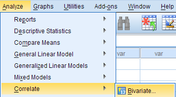
The Bivariate Correlations window opens, where you will specify the variables to be used in the analysis. All of the variables in your dataset appear in the list on the left side. To select variables for the analysis, select the variables in the list on the left and click the blue arrow button to move them to the right, in the Variables field.

A Variables : The variables to be used in the bivariate Pearson Correlation. You must select at least two continuous variables, but may select more than two. The test will produce correlation coefficients for each pair of variables in this list.

B Correlation Coefficients: There are multiple types of correlation coefficients. By default, Pearson is selected. Selecting Pearson will produce the test statistics for a bivariate Pearson Correlation.

C Test of Significance:  Click Two-tailed or One-tailed , depending on your desired significance test. SPSS uses a two-tailed test by default.

D Flag significant correlations: Checking this option will include asterisks (**) next to statistically significant correlations in the output. By default, SPSS marks statistical significance at the alpha = 0.05 and alpha = 0.01 levels, but not at the alpha = 0.001 level (which is treated as alpha = 0.01)

E Options : Clicking Options will open a window where you can specify which Statistics to include (i.e., Means and standard deviations , Cross-product deviations and covariances ) and how to address Missing Values (i.e., Exclude cases pairwise or Exclude cases listwise ). Note that the pairwise/listwise setting does not affect your computations if you are only entering two variable, but can make a very large difference if you are entering three or more variables into the correlation procedure.

Example: Understanding the linear association between weight and height

Problem statement.

Perhaps you would like to test whether there is a statistically significant linear relationship between two continuous variables, weight and height (and by extension, infer whether the association is significant in the population). You can use a bivariate Pearson Correlation to test whether there is a statistically significant linear relationship between height and weight, and to determine the strength and direction of the association.

Before the Test

In the sample data, we will use two variables: “Height” and “Weight.” The variable “Height” is a continuous measure of height in inches and exhibits a range of values from 55.00 to 84.41 ( Analyze > Descriptive Statistics > Descriptives ). The variable “Weight” is a continuous measure of weight in pounds and exhibits a range of values from 101.71 to 350.07.

Before we look at the Pearson correlations, we should look at the scatterplots of our variables to get an idea of what to expect. In particular, we need to determine if it's reasonable to assume that our variables have linear relationships. Click Graphs > Legacy Dialogs > Scatter/Dot . In the Scatter/Dot window, click Simple Scatter , then click Define . Move variable Height to the X Axis box, and move variable Weight to the Y Axis box. When finished, click OK .

To add a linear fit like the one depicted, double-click on the plot in the Output Viewer to open the Chart Editor. Click Elements > Fit Line at Total . In the Properties window, make sure the Fit Method is set to Linear , then click Apply . (Notice that adding the linear regression trend line will also add the R-squared value in the margin of the plot. If we take the square root of this number, it should match the value of the Pearson correlation we obtain.)

From the scatterplot, we can see that as height increases, weight also tends to increase. There does appear to be some linear relationship.

Running the Test

To run the bivariate Pearson Correlation, click  Analyze > Correlate > Bivariate . Select the variables Height and Weight and move them to the Variables box. In the Correlation Coefficients area, select Pearson . In the Test of Significance area, select your desired significance test, two-tailed or one-tailed. We will select a two-tailed significance test in this example. Check the box next to Flag significant correlations .

Click OK to run the bivariate Pearson Correlation. Output for the analysis will display in the Output Viewer.

The results will display the correlations in a table, labeled Correlations .

A Correlation of Height with itself (r=1), and the number of nonmissing observations for height (n=408).

B Correlation of height and weight (r=0.513), based on n=354 observations with pairwise nonmissing values.

C Correlation of height and weight (r=0.513), based on n=354 observations with pairwise nonmissing values.

D Correlation of weight with itself (r=1), and the number of nonmissing observations for weight (n=376).

The important cells we want to look at are either B or C. (Cells B and C are identical, because they include information about the same pair of variables.) Cells B and C contain the correlation coefficient for the correlation between height and weight, its p-value, and the number of complete pairwise observations that the calculation was based on.

The correlations in the main diagonal (cells A and D) are all equal to 1. This is because a variable is always perfectly correlated with itself. Notice, however, that the sample sizes are different in cell A ( n =408) versus cell D ( n =376). This is because of missing data -- there are more missing observations for variable Weight than there are for variable Height.

If you have opted to flag significant correlations, SPSS will mark a 0.05 significance level with one asterisk (*) and a 0.01 significance level with two asterisks (0.01). In cell B (repeated in cell C), we can see that the Pearson correlation coefficient for height and weight is .513, which is significant ( p < .001 for a two-tailed test), based on 354 complete observations (i.e., cases with nonmissing values for both height and weight).

Decision and Conclusions

Based on the results, we can state the following:

• Weight and height have a statistically significant linear relationship ( r =.513, p < .001).
• The direction of the relationship is positive (i.e., height and weight are positively correlated), meaning that these variables tend to increase together (i.e., greater height is associated with greater weight).
• The magnitude, or strength, of the association is approximately moderate (.3 < | r | < .5).
• << Previous: Chi-Square Test of Independence
• Next: One Sample t Test >>
• Last Updated: May 10, 2024 1:32 PM
• URL: https://libguides.library.kent.edu/SPSS

Street Address

Mailing address, quick links.

• How Are We Doing?
• Student Jobs

Information

• Accessibility
• Emergency Information
• For Our Alumni
• For the Media
• Jobs & Employment
• Life at KSU
• Privacy Statement
• Technology Support
• Website Feedback

Want to create or adapt books like this? Learn more about how Pressbooks supports open publishing practices.

Section 4.2: Correlation Assumptions, Interpretation, and Write Up

Learning Objectives

At the end of this section you should be able to answer the following questions:

• What assumptions should be checked before performing a Pearson correlation test?
• What is the relationship between correlation and causation?

Correlation Assumptions

There are four assumptions to check before performing a Pearson correlation test.

• The two variables (the variables of interest) need to be using a continuous scale.
• The two variables of interest should have a linear relationship, which you can check with a scatterplot.
• There should be no spurious outliers.
• The variables should be normally or near-to-normally distributed.

Correlation Interpretation

For this example will be looking at two relationships: levels of physical illness and mental distress, and physical illness and life satisfaction.

PowerPoint: Correlation Output

Have a look at the following slides while you are reviewing this chapter:

• Chapter Four Correlation Output

As you can see from the output ( circled in green ), the relationship between physical illness and mental distress is both a positive and statistically significant. As a person reports higher levels of physical illness, they are more likely to report higher levels of mental distress. The reverse is true of the relationship between physical illness and life satisfaction, with these showing a significant negative relationship ( shown in red ). The greater levels of physical illness, the more likely the person is to have lower levels of life satisfaction. Both relationships are significant (see p values) and are medium in strength.

Although we have two significant relationships or associations between these variables, it does not mean that one variable causes the other. Researchers need to remember that there may be third variable (or covariates) present that affects both variables accounted for in a correlation coefficient. Therefore, the existence of a significant correlation coefficient for a pair of variables by itself does not imply causation between the two variables.

Correlation Write Up

A write-up for a Correlation Analyses should  look like this:

Among Australian Facebook users, the levels of reported physical illness and mental distress showed a medium positive relationship, r (366) = .47, p < .001, whereas the levels of physical illness and life satisfaction showed a medium negative relationship, r (366) = -.34, p < .001.

Statistics for Research Students Copyright © 2022 by University of Southern Queensland is licensed under a Creative Commons Attribution 4.0 International License , except where otherwise noted.

Share This Book

Statistics Made Easy

How to Report Pearson’s r in APA Format (With Examples)

A Pearson Correlation Coefficient , often denoted r , measures the linear association between two variables.

It always takes on a value between -1 and 1 where:

• -1 indicates a perfectly negative linear correlation between two variables
• 0 indicates no linear correlation between two variables
• 1 indicates a perfectly positive linear correlation between two variables

We use the following general structure to report a Pearson’s r in APA format:

A Pearson correlation coefficient was computed to assess the linear relationship between [variable 1] and [variable 2] .   There was a [negative or positive] correlation between the two variables, r( df ) = [r value] , p = [p-value] .

Keep in mind the following when reporting Pearson’s r  in APA format:

• Round the p-value to three decimal places.
• Round the value for r to two decimal places.
• Drop the leading 0 for the p-value and r (e.g. use .77, not 0.77)
• The degrees of freedom (df) is calculated as N – 2.

The following examples show how to report Pearson’s r in APA format in various scenarios.

Example 1: Hours Studied vs. Exam Score Received

A professor collected data for the number of hours studied and the exam score received for 40 students in his class. He found the Pearson correlation coefficient between the two variables to be 0.48 with a corresponding p-value of 0.002.

Here is how to report Pearson’s r in APA format:

A Pearson correlation coefficient was computed to assess the linear relationship between hours studied and exam score.   There was a positive correlation between the two variables, r(38) = .48, p = .002.

Example 2: Time Spent Running vs. Body Fat

A doctor collected data for the number of hours spent running per week and body fat percentage for 35 patients. He found the Pearson correlation coefficient between the two variables to be -0.37 with a corresponding p-value of 0.029.

A Pearson correlation coefficient was computed to assess the linear relationship between hours spent running and body fat percentage.   There was a negative correlation between the two variables, r(33) = -.37, p = .029.

Example 3: Ad Spend vs. Revenue Generated

A company collected data for the amount of money spent on advertising and the total revenue generated during 15 consecutive sales periods. They found the Pearson correlation coefficient between the two variables to be 0.71 with a corresponding p-value of 0.003.

A Pearson correlation coefficient was computed to assess the linear relationship between advertising spend and total revenue.   There was a positive correlation between the two variables, r(13) = .71, p = .003.

Additional Resources

The following tutorials explain how to report other statistical tests and procedures in APA format:

How to Report Cronbach’s Alpha (With Examples) How to Report t-Test Results (With Examples) How to Report Regression Results (With Examples) How to Report ANOVA Results (With Examples)

Featured Posts

Hey there. My name is Zach Bobbitt. I have a Masters of Science degree in Applied Statistics and I’ve worked on machine learning algorithms for professional businesses in both healthcare and retail. I’m passionate about statistics, machine learning, and data visualization and I created Statology to be a resource for both students and teachers alike.  My goal with this site is to help you learn statistics through using simple terms, plenty of real-world examples, and helpful illustrations.

3 Replies to “How to Report Pearson’s r in APA Format (With Examples)”

Your effort here helped remove statistical anxiety for me and my students. Thanks a lot.

what about a p-value that is not significant?

Thank you for writing an interpretation with examples.

Leave a Reply Cancel reply

Your email address will not be published. Required fields are marked *

Join the Statology Community

Sign up to receive Statology's exclusive study resource: 100 practice problems with step-by-step solutions. Plus, get our latest insights, tutorials, and data analysis tips straight to your inbox!

By subscribing you accept Statology's Privacy Policy.

Results Section

The results section is where you tell the reader the basic descriptive information about the scales you used (report the mean and standard deviation for each scale).   If you have more than 3 or 4 variables in your paper, you might want to put this descriptive information in a table to keep the text from being too choppy and bogged down (see the APA manual for ideas on creating good tables).   In the results section, you also tell the reader what statistics you conducted to test your hypothesis (-ses) and what the results indicated.   In this paper, you conducted bivariate correlation(s) to test your hypothesis.

Include in Results (include the following in this order in your results section):

   Give the descriptive statistics for the relevant variables (mean, standard deviation).  

   Provide a brief rephrasing of your hypothesis(es) (avoid exact restatement).   Then tell the reader what statistical test you used to test your hypothesis and what you found.

   Explain which correlations were in the predicted direction, and which were not (if any).   Were differences statistically significant (i.e., p < .05 or below)?   Don't merely give the statistics without any explanation.   Whenever you make a claim that there is (or is not) a significant correlation between X and Y, the reader has to be able to verify it by looking at the appropriate test statistic.   For example do not report “The correlation between private self-consciousness and college adjustment was r = - .26, p < .01.” In general, you should not use numbers as part of a sentence in this way. Instead, interpret important data for the reader and use words throughout your sentences: “The negative correlation between private self-consciousness and college adjustment indicated that the more participants felt self-conscious, the worse their adjustment to college, r = - .26, p < .01”

   However, don't try to interpret why you got the results you did.   Leave that to the Discussion.

   Note : Be sure to underline all abbreviations of test statistics (e.g., M for mean and SD for standard deviation). See pages 112-118 of the APA manual for more on reporting statistics in text.

Some specifics:

     For each correlation, you need to report the following information either in the text of your paper or in a table: correlation coefficient, significance level (p value).  

     If you are reporting a single correlation for the whole results section, report it in the text of the paper as follows:     r =.26, p < .01    or     r = -.11, n.s.

   Use n.s. if not significant; or use whichever of the following is most accurate:

              p < .05;   p < .01;   p < .001

   If your correlation was non significant, but p < .10 you can still talk about it.   You might put the following text in your paper:   “While the correlation was not significant relative to the standard alpha level of .05, the p-value was less than .10.” Then provide a rationale for why you should still be able to discuss this non-significant correlation (see your hypothesis testing lecture notes).   You may then cautiously interpret such a correlation. Don’t make grand conclusions or use strong language based on the existence of a marginally significant finding. Also, you should indicate that a marginal correlation is non -significant in a table; only refer to the correlation as “approaching significance” in the text of the paper .

If you computed two or more correlations (thus involving at least three variables) provide a   table at the end of the paper (ordinarily tables would only be used for even more complex findings, but I'd like you to practice since you have a few correlations to work with).   Create a correlation matrix like the example (see Table 1).   If you include a correlation matrix table, you should, in the text of the result section, refer readers to your table instead of typing out the r and the p value for each correlation. If you are using Word as your word processor, create the table, then you can adjust the "borders and shading" for each cell/row/column to get the table formatted properly.   I can show you how if you have trouble. Other word processors should have similar functions.

This Table is an Example of a Correlation Matrix among Three Variables for an Imaginary Sample of College Students (n = 129).

* p < .05;   **p < .01

=====================================================================

You need to report the statistics in some way in your result section, but regardless of whether you use a table or type the statistics in the text, you should also interpret the correlation for the reader… say exactly what that means:

E.g.   “As expected, college adjustment was positively correlated with the amount of contact with friends and family members (see Table 1).”   

E.g.   “No significant relationship was found between the importance of one's social life and social adjustment to college, r = -.11, n.s.

E.g.   “As shown in Table 1, some of my predictions were supported.   There was a significant correlation between extroversion and life satisfaction.   However, life satisfaction was not significantly related to college adjustment.”

See your text, APA manual, and Sample Paper (“The Title of the Paper”) for more information and suggestions.   In general, I would suggest writing the words of the results section first, and then going back to insert the numbers and statistical information.

Discussion section

In your discussion section, relate the results back to your initial hypotheses.   Do they support or disconfirm them?   Remember: Results do not prove hypotheses right or wrong, they support them or fail to provide support for them.

I suggest the following information in the following order:

   Provide a very brief summary of the most important parts of the introduction and then the results sections. In doing so, you should relate the results to the theories you introduced in the Introduction. Your findings are just one piece among many -- resist the tendency to make your results the final story about the   phenomenon or theory of interest.   Integrate the results and try to make sense of the pattern of the findings.

   In the case of a correlational project, be careful to not use causal language to discuss your results – unless you did an experiment you cannot infer causality. However, it would be impossible to fully discuss the implications of your results without making reference to causality. That is fine. Just don't claim that your results themselves are demonstrating causality.

   If your findings did not support your hypotheses, speculate why that might be so.   You might reconsider the logic of your hypotheses.   Or, reconsider whether the variables are adequately measuring the relationship.   For example, if you hypothesized a relationship between anger toward the stigmatized and narcissism and didn’t find it – consider whether anger is really the right variable... perhaps "disgust" would better capture the relationship. Alternatively, you might also consider whether the relationship you hypothesized might only show up in certain populations of people or under certain conditions (e.g., self-threat). Where possible, support your speculation with references.

   Talk about any qualifications important to your findings (all studies have weaknesses/qualifications). This includes alternative explanations for the results.   For example, you might speculate about an unexamined third variable that was not present in you study.   However, BE SPECIFIC and back up any assertions you make.   For example, if you claim that 3 rd variables might affect your correlations, tell me what they are and how they would affect your correlations.

   Speculate about future directions that research could take to further investigate your question. This might relate back to any weaknesses you’ve mentioned above (or reasons why the results didn’t turn out as expected).   Future directions may also include interesting next steps in the research.

   A discussion section is about “what we have learned so far”; and “where we should go next”;   Your final conclusion should talk briefly about the broader significance of your findings.   What do they imply about human nature or some aspect of it? (Don't wildly speculate, however!) Leave the reader feeling like this is an important topic... you will likely refer back to your opening paragraph of the introduction here and have partial answers or more specific responses to the questions you posed.

Important Parts of the Paper – Don’t Forget Them!!

Title page -   Try to write a title that maximally informs the reader about the topic, without being ridiculously long. Use titles of articles you've read as examples of form. Also provide the RUNNING HEAD and an abbreviated title that appears in the header of each page along with the page number. Provide your name and institutional affiliation (Hanover College). See APA Manual and sample paper.

Abstract - Write the abstract LAST. An abstract is a super-short summary and is difficult to write.

Info on abstracts from APA manual:

An abstract is a brief, comprehensive summary of the contents of an article, allowing readers to survey the contents quickly.

A good abstract is:

   accurate : Ensure that your abstract correctly reflects the purpose and content of your paper.   Do not include information that does not appear in the body of the paper.

   self-contained :   Define all abbreviations and acronyms.   Spell out names of tests/ questionnaires.   Define unique terms.   Paraphrase rather than quote.  

   concise and specific : Make each sentence maximally informative, especially the lead sentence.   Begin the abstract with the most important information (your question), but do not repeat the title.   Be as brief as possible.

   non-evaluative : Report rather than evaluate: do not add to or comment on what is in the body of the manuscript.

   coherent and readable : Write in clear and vigorous prose. Use the third person rather than the first person.

In less than 150 words your abstract should describe:

   the problem under investigation (an "introduction" type sentence)

   the specific variables investigated and the method of doing so (a "method" type sentence)

   the results of the study in brief (no numbers, just words)

   a hint about the general direction the discussion section takes

References : Use APA style.   See your APA manual, textbook and the sample paper for examples of how to cite and how to make a reference list.   Make sure that all references mentioned in the text are also mentioned in the reference list and vice versa.

Tables and/or Figures :   Use APA style. Tables go at the very end of your paper.   Make sure you refer to the table or figure in the text of your paper.  

*See APA Manual, textbook and sample paper for information on how to format each section of your paper and how to order the sections.

• school Campus Bookshelves
• menu_book Bookshelves
• perm_media Learning Objects
• login Login
• how_to_reg Request Instructor Account
• hub Instructor Commons

Margin Size

• Download Page (PDF)
• Download Full Book (PDF)
• Periodic Table
• Physics Constants
• Scientific Calculator
• Reference & Cite
• Tools expand_more
• Readability

selected template will load here

This action is not available.

12.5: Testing the Significance of the Correlation Coefficient

• Last updated
• Save as PDF
• Page ID 800

\( \newcommand{\vecs}[1]{\overset { \scriptstyle \rightharpoonup} {\mathbf{#1}} } \)

\( \newcommand{\vecd}[1]{\overset{-\!-\!\rightharpoonup}{\vphantom{a}\smash {#1}}} \)

\( \newcommand{\id}{\mathrm{id}}\) \( \newcommand{\Span}{\mathrm{span}}\)

( \newcommand{\kernel}{\mathrm{null}\,}\) \( \newcommand{\range}{\mathrm{range}\,}\)

\( \newcommand{\RealPart}{\mathrm{Re}}\) \( \newcommand{\ImaginaryPart}{\mathrm{Im}}\)

\( \newcommand{\Argument}{\mathrm{Arg}}\) \( \newcommand{\norm}[1]{\| #1 \|}\)

\( \newcommand{\inner}[2]{\langle #1, #2 \rangle}\)

\( \newcommand{\Span}{\mathrm{span}}\)

\( \newcommand{\id}{\mathrm{id}}\)

\( \newcommand{\kernel}{\mathrm{null}\,}\)

\( \newcommand{\range}{\mathrm{range}\,}\)

\( \newcommand{\RealPart}{\mathrm{Re}}\)

\( \newcommand{\ImaginaryPart}{\mathrm{Im}}\)

\( \newcommand{\Argument}{\mathrm{Arg}}\)

\( \newcommand{\norm}[1]{\| #1 \|}\)

\( \newcommand{\Span}{\mathrm{span}}\) \( \newcommand{\AA}{\unicode[.8,0]{x212B}}\)

\( \newcommand{\vectorA}[1]{\vec{#1}}      % arrow\)

\( \newcommand{\vectorAt}[1]{\vec{\text{#1}}}      % arrow\)

\( \newcommand{\vectorB}[1]{\overset { \scriptstyle \rightharpoonup} {\mathbf{#1}} } \)

\( \newcommand{\vectorC}[1]{\textbf{#1}} \)

\( \newcommand{\vectorD}[1]{\overrightarrow{#1}} \)

\( \newcommand{\vectorDt}[1]{\overrightarrow{\text{#1}}} \)

\( \newcommand{\vectE}[1]{\overset{-\!-\!\rightharpoonup}{\vphantom{a}\smash{\mathbf {#1}}}} \)

The correlation coefficient, \(r\), tells us about the strength and direction of the linear relationship between \(x\) and \(y\). However, the reliability of the linear model also depends on how many observed data points are in the sample. We need to look at both the value of the correlation coefficient \(r\) and the sample size \(n\), together. We perform a hypothesis test of the "significance of the correlation coefficient" to decide whether the linear relationship in the sample data is strong enough to use to model the relationship in the population.

The sample data are used to compute \(r\), the correlation coefficient for the sample. If we had data for the entire population, we could find the population correlation coefficient. But because we have only sample data, we cannot calculate the population correlation coefficient. The sample correlation coefficient, \(r\), is our estimate of the unknown population correlation coefficient.

• The symbol for the population correlation coefficient is \(\rho\), the Greek letter "rho."
• \(\rho =\) population correlation coefficient (unknown)
• \(r =\) sample correlation coefficient (known; calculated from sample data)

The hypothesis test lets us decide whether the value of the population correlation coefficient \(\rho\) is "close to zero" or "significantly different from zero". We decide this based on the sample correlation coefficient \(r\) and the sample size \(n\).

If the test concludes that the correlation coefficient is significantly different from zero, we say that the correlation coefficient is "significant."

• Conclusion: There is sufficient evidence to conclude that there is a significant linear relationship between \(x\) and \(y\) because the correlation coefficient is significantly different from zero.
• What the conclusion means: There is a significant linear relationship between \(x\) and \(y\). We can use the regression line to model the linear relationship between \(x\) and \(y\) in the population.

If the test concludes that the correlation coefficient is not significantly different from zero (it is close to zero), we say that correlation coefficient is "not significant".

• Conclusion: "There is insufficient evidence to conclude that there is a significant linear relationship between \(x\) and \(y\) because the correlation coefficient is not significantly different from zero."
• What the conclusion means: There is not a significant linear relationship between \(x\) and \(y\). Therefore, we CANNOT use the regression line to model a linear relationship between \(x\) and \(y\) in the population.
• If \(r\) is significant and the scatter plot shows a linear trend, the line can be used to predict the value of \(y\) for values of \(x\) that are within the domain of observed \(x\) values.
• If \(r\) is not significant OR if the scatter plot does not show a linear trend, the line should not be used for prediction.
• If \(r\) is significant and if the scatter plot shows a linear trend, the line may NOT be appropriate or reliable for prediction OUTSIDE the domain of observed \(x\) values in the data.

PERFORMING THE HYPOTHESIS TEST

• Null Hypothesis: \(H_{0}: \rho = 0\)
• Alternate Hypothesis: \(H_{a}: \rho \neq 0\)

WHAT THE HYPOTHESES MEAN IN WORDS:

• Null Hypothesis \(H_{0}\) : The population correlation coefficient IS NOT significantly different from zero. There IS NOT a significant linear relationship(correlation) between \(x\) and \(y\) in the population.
• Alternate Hypothesis \(H_{a}\) : The population correlation coefficient IS significantly DIFFERENT FROM zero. There IS A SIGNIFICANT LINEAR RELATIONSHIP (correlation) between \(x\) and \(y\) in the population.

DRAWING A CONCLUSION:There are two methods of making the decision. The two methods are equivalent and give the same result.

• Method 1: Using the \(p\text{-value}\)
• Method 2: Using a table of critical values

In this chapter of this textbook, we will always use a significance level of 5%, \(\alpha = 0.05\)

Using the \(p\text{-value}\) method, you could choose any appropriate significance level you want; you are not limited to using \(\alpha = 0.05\). But the table of critical values provided in this textbook assumes that we are using a significance level of 5%, \(\alpha = 0.05\). (If we wanted to use a different significance level than 5% with the critical value method, we would need different tables of critical values that are not provided in this textbook.)

METHOD 1: Using a \(p\text{-value}\) to make a decision

Using the ti83, 83+, 84, 84+ calculator.

To calculate the \(p\text{-value}\) using LinRegTTEST:

On the LinRegTTEST input screen, on the line prompt for \(\beta\) or \(\rho\), highlight "\(\neq 0\)"

The output screen shows the \(p\text{-value}\) on the line that reads "\(p =\)".

(Most computer statistical software can calculate the \(p\text{-value}\).)

If the \(p\text{-value}\) is less than the significance level ( \(\alpha = 0.05\) ):

• Decision: Reject the null hypothesis.
• Conclusion: "There is sufficient evidence to conclude that there is a significant linear relationship between \(x\) and \(y\) because the correlation coefficient is significantly different from zero."

If the \(p\text{-value}\) is NOT less than the significance level ( \(\alpha = 0.05\) )

• Decision: DO NOT REJECT the null hypothesis.
• Conclusion: "There is insufficient evidence to conclude that there is a significant linear relationship between \(x\) and \(y\) because the correlation coefficient is NOT significantly different from zero."

Calculation Notes:

• You will use technology to calculate the \(p\text{-value}\). The following describes the calculations to compute the test statistics and the \(p\text{-value}\):
• The \(p\text{-value}\) is calculated using a \(t\)-distribution with \(n - 2\) degrees of freedom.
• The formula for the test statistic is \(t = \frac{r\sqrt{n-2}}{\sqrt{1-r^{2}}}\). The value of the test statistic, \(t\), is shown in the computer or calculator output along with the \(p\text{-value}\). The test statistic \(t\) has the same sign as the correlation coefficient \(r\).
• The \(p\text{-value}\) is the combined area in both tails.

An alternative way to calculate the \(p\text{-value}\) ( \(p\) ) given by LinRegTTest is the command 2*tcdf(abs(t),10^99, n-2) in 2nd DISTR.

THIRD-EXAM vs FINAL-EXAM EXAMPLE: \(p\text{-value}\) method

• Consider the third exam/final exam example.
• The line of best fit is: \(\hat{y} = -173.51 + 4.83x\) with \(r = 0.6631\) and there are \(n = 11\) data points.
• Can the regression line be used for prediction? Given a third exam score ( \(x\) value), can we use the line to predict the final exam score (predicted \(y\) value)?
• \(H_{0}: \rho = 0\)
• \(H_{a}: \rho \neq 0\)
• \(\alpha = 0.05\)
• The \(p\text{-value}\) is 0.026 (from LinRegTTest on your calculator or from computer software).
• The \(p\text{-value}\), 0.026, is less than the significance level of \(\alpha = 0.05\).
• Decision: Reject the Null Hypothesis \(H_{0}\)
• Conclusion: There is sufficient evidence to conclude that there is a significant linear relationship between the third exam score (\(x\)) and the final exam score (\(y\)) because the correlation coefficient is significantly different from zero.

Because \(r\) is significant and the scatter plot shows a linear trend, the regression line can be used to predict final exam scores.

METHOD 2: Using a table of Critical Values to make a decision

The 95% Critical Values of the Sample Correlation Coefficient Table can be used to give you a good idea of whether the computed value of \(r\) is significant or not . Compare \(r\) to the appropriate critical value in the table. If \(r\) is not between the positive and negative critical values, then the correlation coefficient is significant. If \(r\) is significant, then you may want to use the line for prediction.

Example \(\PageIndex{1}\)

Suppose you computed \(r = 0.801\) using \(n = 10\) data points. \(df = n - 2 = 10 - 2 = 8\). The critical values associated with \(df = 8\) are \(-0.632\) and \(+0.632\). If \(r <\) negative critical value or \(r >\) positive critical value, then \(r\) is significant. Since \(r = 0.801\) and \(0.801 > 0.632\), \(r\) is significant and the line may be used for prediction. If you view this example on a number line, it will help you.

Exercise \(\PageIndex{1}\)

For a given line of best fit, you computed that \(r = 0.6501\) using \(n = 12\) data points and the critical value is 0.576. Can the line be used for prediction? Why or why not?

If the scatter plot looks linear then, yes, the line can be used for prediction, because \(r >\) the positive critical value.

Example \(\PageIndex{2}\)

Suppose you computed \(r = –0.624\) with 14 data points. \(df = 14 – 2 = 12\). The critical values are \(-0.532\) and \(0.532\). Since \(-0.624 < -0.532\), \(r\) is significant and the line can be used for prediction

Exercise \(\PageIndex{2}\)

For a given line of best fit, you compute that \(r = 0.5204\) using \(n = 9\) data points, and the critical value is \(0.666\). Can the line be used for prediction? Why or why not?

No, the line cannot be used for prediction, because \(r <\) the positive critical value.

Example \(\PageIndex{3}\)

Suppose you computed \(r = 0.776\) and \(n = 6\). \(df = 6 - 2 = 4\). The critical values are \(-0.811\) and \(0.811\). Since \(-0.811 < 0.776 < 0.811\), \(r\) is not significant, and the line should not be used for prediction.

Exercise \(\PageIndex{3}\)

For a given line of best fit, you compute that \(r = -0.7204\) using \(n = 8\) data points, and the critical value is \(= 0.707\). Can the line be used for prediction? Why or why not?

Yes, the line can be used for prediction, because \(r <\) the negative critical value.

THIRD-EXAM vs FINAL-EXAM EXAMPLE: critical value method

Consider the third exam/final exam example. The line of best fit is: \(\hat{y} = -173.51 + 4.83x\) with \(r = 0.6631\) and there are \(n = 11\) data points. Can the regression line be used for prediction? Given a third-exam score ( \(x\) value), can we use the line to predict the final exam score (predicted \(y\) value)?

• Use the "95% Critical Value" table for \(r\) with \(df = n - 2 = 11 - 2 = 9\).
• The critical values are \(-0.602\) and \(+0.602\)
• Since \(0.6631 > 0.602\), \(r\) is significant.
• Conclusion:There is sufficient evidence to conclude that there is a significant linear relationship between the third exam score (\(x\)) and the final exam score (\(y\)) because the correlation coefficient is significantly different from zero.

Example \(\PageIndex{4}\)

Suppose you computed the following correlation coefficients. Using the table at the end of the chapter, determine if \(r\) is significant and the line of best fit associated with each r can be used to predict a \(y\) value. If it helps, draw a number line.

• \(r = –0.567\) and the sample size, \(n\), is \(19\). The \(df = n - 2 = 17\). The critical value is \(-0.456\). \(-0.567 < -0.456\) so \(r\) is significant.
• \(r = 0.708\) and the sample size, \(n\), is \(9\). The \(df = n - 2 = 7\). The critical value is \(0.666\). \(0.708 > 0.666\) so \(r\) is significant.
• \(r = 0.134\) and the sample size, \(n\), is \(14\). The \(df = 14 - 2 = 12\). The critical value is \(0.532\). \(0.134\) is between \(-0.532\) and \(0.532\) so \(r\) is not significant.
• \(r = 0\) and the sample size, \(n\), is five. No matter what the \(dfs\) are, \(r = 0\) is between the two critical values so \(r\) is not significant.

Exercise \(\PageIndex{4}\)

For a given line of best fit, you compute that \(r = 0\) using \(n = 100\) data points. Can the line be used for prediction? Why or why not?

No, the line cannot be used for prediction no matter what the sample size is.

Assumptions in Testing the Significance of the Correlation Coefficient

Testing the significance of the correlation coefficient requires that certain assumptions about the data are satisfied. The premise of this test is that the data are a sample of observed points taken from a larger population. We have not examined the entire population because it is not possible or feasible to do so. We are examining the sample to draw a conclusion about whether the linear relationship that we see between \(x\) and \(y\) in the sample data provides strong enough evidence so that we can conclude that there is a linear relationship between \(x\) and \(y\) in the population.

The regression line equation that we calculate from the sample data gives the best-fit line for our particular sample. We want to use this best-fit line for the sample as an estimate of the best-fit line for the population. Examining the scatter plot and testing the significance of the correlation coefficient helps us determine if it is appropriate to do this.

The assumptions underlying the test of significance are:

• There is a linear relationship in the population that models the average value of \(y\) for varying values of \(x\). In other words, the expected value of \(y\) for each particular value lies on a straight line in the population. (We do not know the equation for the line for the population. Our regression line from the sample is our best estimate of this line in the population.)
• The \(y\) values for any particular \(x\) value are normally distributed about the line. This implies that there are more \(y\) values scattered closer to the line than are scattered farther away. Assumption (1) implies that these normal distributions are centered on the line: the means of these normal distributions of \(y\) values lie on the line.
• The standard deviations of the population \(y\) values about the line are equal for each value of \(x\). In other words, each of these normal distributions of \(y\) values has the same shape and spread about the line.
• The residual errors are mutually independent (no pattern).
• The data are produced from a well-designed, random sample or randomized experiment.

Linear regression is a procedure for fitting a straight line of the form \(\hat{y} = a + bx\) to data. The conditions for regression are:

• Linear In the population, there is a linear relationship that models the average value of \(y\) for different values of \(x\).
• Independent The residuals are assumed to be independent.
• Normal The \(y\) values are distributed normally for any value of \(x\).
• Equal variance The standard deviation of the \(y\) values is equal for each \(x\) value.
• Random The data are produced from a well-designed random sample or randomized experiment.

The slope \(b\) and intercept \(a\) of the least-squares line estimate the slope \(\beta\) and intercept \(\alpha\) of the population (true) regression line. To estimate the population standard deviation of \(y\), \(\sigma\), use the standard deviation of the residuals, \(s\). \(s = \sqrt{\frac{SEE}{n-2}}\). The variable \(\rho\) (rho) is the population correlation coefficient. To test the null hypothesis \(H_{0}: \rho =\) hypothesized value , use a linear regression t-test. The most common null hypothesis is \(H_{0}: \rho = 0\) which indicates there is no linear relationship between \(x\) and \(y\) in the population. The TI-83, 83+, 84, 84+ calculator function LinRegTTest can perform this test (STATS TESTS LinRegTTest).

Formula Review

Least Squares Line or Line of Best Fit:

\[\hat{y} = a + bx\]

\[a = y\text{-intercept}\]

\[b = \text{slope}\]

Standard deviation of the residuals:

\[s = \sqrt{\frac{SSE}{n-2}}\]

\[SSE = \text{sum of squared errors}\]

\[n = \text{the number of data points}\]

More From Forbes

3 psychologist-approved habits that lead to relationship success.

• Share to Facebook
• Share to Twitter
• Share to Linkedin

The little things—often overlooked—can significantly enhance the quality and longevity of a ... [+] partnership.

When discussing relationship success, we often hear about the same key ingredients and concepts that dominate the conversation. Communication is hailed as the cornerstone of any relationship, emphasizing the need for open dialogue and active listening. Sex is often discussed in terms of its frequency and quality, viewed as a barometer of relational health. Trust is highlighted as the glue that holds partners together, leading to a sense of security and stability.

These elements are undeniably important, but they are so frequently mentioned that they can sometimes overshadow the subtler, yet equally vital, habits that contribute to a thriving relationship. Focusing exclusively on the usual macro elements can lead to an incomplete picture of what makes a relationship truly successful. It’s important to remember that relationships are dynamic and multifaceted, requiring more than just these fundamental elements. The everyday nuances and seemingly minor practices can have profound effects on relationship satisfaction. Here are three such practices that deserve more attention.

1. Incorporating A Sense Of Playfulness

Playfulness in a relationship might sound frivolous, but it plays a critical role in maintaining a joyful and resilient partnership. Engaging in playful behavior helps partners bond, reduce stress and maintain a sense of spontaneity and excitement. According to a study published in Social and Personality Psychology Compass, playfulness contributes to relationship satisfaction, reduces conflict, mitigates monotony and builds trust—implying that playfulness indirectly supports relationship longevity, happiness and stability. Here’s how to cultivate this habit:

• Spontaneity. Incorporate spontaneous activities into your routine. Surprise your partner with an impromptu date night or a spontaneous weekend getaway. These unexpected moments can break the monotony of daily life and reignite the excitement in your relationship. Even simple acts, like leaving a surprise note or planning an unexpected outing, can inject a sense of adventure and joy into your daily interactions.
• Humor. Share jokes, laugh together and don’t be afraid to be silly. Humor can diffuse tension, create a sense of closeness and keep the relationship lighthearted. Watch a comedy show, share funny memes or reminisce about humorous moments you’ve experienced together. The act of laughing together not only releases endorphins but also strengthens your bond by creating positive associations and memories.
• Role-playing and imaginary scenarios. Occasionally indulge in role-playing or create imaginary scenarios. Pretend to be characters from your favorite movies, or imagine you’re on a deserted island and have to come up with survival strategies. These playful exercises can help you tap into your creative sides, encourage problem-solving together and add an element of fantasy and fun to your relationship.

Samsung Slashes Galaxy S24 Price In A Major New Promotion

This is your last chance to shop these 114 best memorial day sales, get up to 50 off during the hoka memorial day sale, 2. following rituals and traditions.

A study conducted at the University of Illinois highlights the significant role of rituals, such as holiday celebrations and shared activities, in dating relationships. The practice of engaging in rituals helps couples learn more about each other and serves as a diagnostic tool for the relationship’s future.

For instance, rituals bond individuals, provide insights into couple dynamics, impact communication and offer new perspectives on the relationship. They can strengthen commitment or highlight conflicts, influencing the likelihood of marriage. Additionally, rituals encourage partners to pause and reflect, helping them understand their identity as a couple and potential family.

Here are several ways to incorporate meaningful rituals and traditions into your relationship:

• Weekly rituals. Establish consistent weekly activities that you both enjoy. This could be a Saturday morning breakfast ritual, a Friday movie night where you take turns choosing films or a Sunday afternoon walk in a nearby park. These routines provide stability and a sense of regular, reliable connection.
• Seasonal traditions. Create traditions around holidays and changing seasons. Decorating the house together for holidays, planning an annual trip or engaging in seasonal activities like apple picking in the fall or planting a garden in the spring, create a rhythm that ties your relationship to the natural cycles of the year, enhancing your connection to each other and the world around you.
• Daily connection points. Incorporate small, daily rituals to maintain a sense of closeness amidst the hustle and bustle of everyday life. Morning coffee together, sharing a few minutes to talk about your day before bed or a daily text message to check in on each other ensure that you stay connected and provide consistent opportunities for communication and support.

3. Practicing Gratitude As A Team

Gratitude is often discussed in the context of individual well-being, but practicing it as a team can significantly enhance relationship satisfaction. According to a study published in Personal Relationships , gratitude positively impacts relationships, leading to increased feelings of connection and satisfaction for both the giver and the receiver the following day. Expressing gratitude together helps maintain a positive perspective and reinforces the value each partner brings to the relationship.

Here’s how to practice this habit:

• Gratitude journal. Keep a joint gratitude journal where both partners write down things they are thankful for about each other and their relationship. Set aside time each week to jot down your thoughts, focusing on small daily gestures and significant acts of love and support. Reviewing the journal together periodically can reinforce positive feelings and remind you of the many reasons you appreciate each other. This practice highlights the good in your relationship and creates a tangible record of your journey together.
• Thank you notes . Leave spontaneous thank-you notes for each other, expressing appreciation for both small and significant gestures. These notes can be simple yet impactful, such as thanking your partner for doing the dishes, offering emotional support or simply being there when you needed a hug. The act of writing and receiving thank-you notes fosters a habit of noticing and appreciating the little things that often go unnoticed. Place these notes in unexpected places like on the bathroom mirror, inside a lunchbox or under a pillow to bring a smile to your partner’s face and brighten their day.

While communication, sex and trust are fundamental to a healthy relationship, it’s the smaller, often overlooked habits that can truly enhance relational satisfaction. By paying attention to these lesser-known habits, you can build a stronger, more fulfilling relationship that stands the test of time.

Is your relationship working on both the macro and micro levels? Take the Relationship Satisfaction Scale to know more.

• Editorial Standards
• Reprints & Permissions

Join The Conversation

One Community. Many Voices. Create a free account to share your thoughts. 

Forbes Community Guidelines

Our community is about connecting people through open and thoughtful conversations. We want our readers to share their views and exchange ideas and facts in a safe space.

In order to do so, please follow the posting rules in our site's  Terms of Service.   We've summarized some of those key rules below. Simply put, keep it civil.

Your post will be rejected if we notice that it seems to contain:

• False or intentionally out-of-context or misleading information
• Insults, profanity, incoherent, obscene or inflammatory language or threats of any kind
• Attacks on the identity of other commenters or the article's author
• Content that otherwise violates our site's  terms.

User accounts will be blocked if we notice or believe that users are engaged in:

• Continuous attempts to re-post comments that have been previously moderated/rejected
• Racist, sexist, homophobic or other discriminatory comments
• Attempts or tactics that put the site security at risk
• Actions that otherwise violate our site's  terms.

So, how can you be a power user?

• Stay on topic and share your insights
• Feel free to be clear and thoughtful to get your point across
• ‘Like’ or ‘Dislike’ to show your point of view.
• Protect your community.
• Use the report tool to alert us when someone breaks the rules.

Thanks for reading our community guidelines. Please read the full list of posting rules found in our site's  Terms of Service.