hypothesis testing 9 steps

• Comprehensive Learning Paths
• 150+ Hours of Videos
• Complete Access to Jupyter notebooks, Datasets, References.

Hypothesis Testing – A Deep Dive into Hypothesis Testing, The Backbone of Statistical Inference

• September 21, 2023

Explore the intricacies of hypothesis testing, a cornerstone of statistical analysis. Dive into methods, interpretations, and applications for making data-driven decisions.

In this Blog post we will learn:

• What is Hypothesis Testing?
• Steps in Hypothesis Testing 2.1. Set up Hypotheses: Null and Alternative 2.2. Choose a Significance Level (α) 2.3. Calculate a test statistic and P-Value 2.4. Make a Decision
• Example : Testing a new drug.
• Example in python

1. What is Hypothesis Testing?

In simple terms, hypothesis testing is a method used to make decisions or inferences about population parameters based on sample data. Imagine being handed a dice and asked if it’s biased. By rolling it a few times and analyzing the outcomes, you’d be engaging in the essence of hypothesis testing.

Think of hypothesis testing as the scientific method of the statistics world. Suppose you hear claims like “This new drug works wonders!” or “Our new website design boosts sales.” How do you know if these statements hold water? Enter hypothesis testing.

2. Steps in Hypothesis Testing

• Set up Hypotheses : Begin with a null hypothesis (H0) and an alternative hypothesis (Ha).
• Choose a Significance Level (α) : Typically 0.05, this is the probability of rejecting the null hypothesis when it’s actually true. Think of it as the chance of accusing an innocent person.
• Calculate Test statistic and P-Value : Gather evidence (data) and calculate a test statistic.
• p-value : This is the probability of observing the data, given that the null hypothesis is true. A small p-value (typically ≤ 0.05) suggests the data is inconsistent with the null hypothesis.
• Decision Rule : If the p-value is less than or equal to α, you reject the null hypothesis in favor of the alternative.

2.1. Set up Hypotheses: Null and Alternative

Before diving into testing, we must formulate hypotheses. The null hypothesis (H0) represents the default assumption, while the alternative hypothesis (H1) challenges it.

For instance, in drug testing, H0 : “The new drug is no better than the existing one,” H1 : “The new drug is superior .”

2.2. Choose a Significance Level (α)

When You collect and analyze data to test H0 and H1 hypotheses. Based on your analysis, you decide whether to reject the null hypothesis in favor of the alternative, or fail to reject / Accept the null hypothesis.

The significance level, often denoted by $α$, represents the probability of rejecting the null hypothesis when it is actually true.

In other words, it’s the risk you’re willing to take of making a Type I error (false positive).

Type I Error (False Positive) :

• Symbolized by the Greek letter alpha (α).
• Occurs when you incorrectly reject a true null hypothesis . In other words, you conclude that there is an effect or difference when, in reality, there isn’t.
• The probability of making a Type I error is denoted by the significance level of a test. Commonly, tests are conducted at the 0.05 significance level , which means there’s a 5% chance of making a Type I error .
• Commonly used significance levels are 0.01, 0.05, and 0.10, but the choice depends on the context of the study and the level of risk one is willing to accept.

Example : If a drug is not effective (truth), but a clinical trial incorrectly concludes that it is effective (based on the sample data), then a Type I error has occurred.

Type II Error (False Negative) :

• Symbolized by the Greek letter beta (β).
• Occurs when you accept a false null hypothesis . This means you conclude there is no effect or difference when, in reality, there is.
• The probability of making a Type II error is denoted by β. The power of a test (1 – β) represents the probability of correctly rejecting a false null hypothesis.

Example : If a drug is effective (truth), but a clinical trial incorrectly concludes that it is not effective (based on the sample data), then a Type II error has occurred.

Balancing the Errors :

In practice, there’s a trade-off between Type I and Type II errors. Reducing the risk of one typically increases the risk of the other. For example, if you want to decrease the probability of a Type I error (by setting a lower significance level), you might increase the probability of a Type II error unless you compensate by collecting more data or making other adjustments.

It’s essential to understand the consequences of both types of errors in any given context. In some situations, a Type I error might be more severe, while in others, a Type II error might be of greater concern. This understanding guides researchers in designing their experiments and choosing appropriate significance levels.

2.3. Calculate a test statistic and P-Value

Test statistic : A test statistic is a single number that helps us understand how far our sample data is from what we’d expect under a null hypothesis (a basic assumption we’re trying to test against). Generally, the larger the test statistic, the more evidence we have against our null hypothesis. It helps us decide whether the differences we observe in our data are due to random chance or if there’s an actual effect.

P-value : The P-value tells us how likely we would get our observed results (or something more extreme) if the null hypothesis were true. It’s a value between 0 and 1. – A smaller P-value (typically below 0.05) means that the observation is rare under the null hypothesis, so we might reject the null hypothesis. – A larger P-value suggests that what we observed could easily happen by random chance, so we might not reject the null hypothesis.

2.4. Make a Decision

Relationship between $α$ and P-Value

When conducting a hypothesis test:

We then calculate the p-value from our sample data and the test statistic.

Finally, we compare the p-value to our chosen $α$:

• If $p−value≤α$: We reject the null hypothesis in favor of the alternative hypothesis. The result is said to be statistically significant.
• If $p−value>α$: We fail to reject the null hypothesis. There isn’t enough statistical evidence to support the alternative hypothesis.

3. Example : Testing a new drug.

Imagine we are investigating whether a new drug is effective at treating headaches faster than drug B.

Setting Up the Experiment : You gather 100 people who suffer from headaches. Half of them (50 people) are given the new drug (let’s call this the ‘Drug Group’), and the other half are given a sugar pill, which doesn’t contain any medication.

• Set up Hypotheses : Before starting, you make a prediction:
• Null Hypothesis (H0): The new drug has no effect. Any difference in healing time between the two groups is just due to random chance.
• Alternative Hypothesis (H1): The new drug does have an effect. The difference in healing time between the two groups is significant and not just by chance.

Calculate Test statistic and P-Value : After the experiment, you analyze the data. The “test statistic” is a number that helps you understand the difference between the two groups in terms of standard units.

For instance, let’s say:

• The average healing time in the Drug Group is 2 hours.
• The average healing time in the Placebo Group is 3 hours.

The test statistic helps you understand how significant this 1-hour difference is. If the groups are large and the spread of healing times in each group is small, then this difference might be significant. But if there’s a huge variation in healing times, the 1-hour difference might not be so special.

Imagine the P-value as answering this question: “If the new drug had NO real effect, what’s the probability that I’d see a difference as extreme (or more extreme) as the one I found, just by random chance?”

For instance:

• P-value of 0.01 means there’s a 1% chance that the observed difference (or a more extreme difference) would occur if the drug had no effect. That’s pretty rare, so we might consider the drug effective.
• P-value of 0.5 means there’s a 50% chance you’d see this difference just by chance. That’s pretty high, so we might not be convinced the drug is doing much.
• If the P-value is less than ($α$) 0.05: the results are “statistically significant,” and they might reject the null hypothesis , believing the new drug has an effect.
• If the P-value is greater than ($α$) 0.05: the results are not statistically significant, and they don’t reject the null hypothesis , remaining unsure if the drug has a genuine effect.

4. Example in python

For simplicity, let’s say we’re using a t-test (common for comparing means). Let’s dive into Python:

Making a Decision : “The results are statistically significant! p-value < 0.05 , The drug seems to have an effect!” If not, we’d say, “Looks like the drug isn’t as miraculous as we thought.”

5. Conclusion

Hypothesis testing is an indispensable tool in data science, allowing us to make data-driven decisions with confidence. By understanding its principles, conducting tests properly, and considering real-world applications, you can harness the power of hypothesis testing to unlock valuable insights from your data.

More Articles

Correlation – connecting the dots, the role of correlation in data analysis, sampling and sampling distributions – a comprehensive guide on sampling and sampling distributions, law of large numbers – a deep dive into the world of statistics, central limit theorem – a deep dive into central limit theorem and its significance in statistics, skewness and kurtosis – peaks and tails, understanding data through skewness and kurtosis”, similar articles, complete introduction to linear regression in r, how to implement common statistical significance tests and find the p value, logistic regression – a complete tutorial with examples in r.

Subscribe to Machine Learning Plus for high value data science content

© Machinelearningplus. All rights reserved.

Machine Learning A-Z™: Hands-On Python & R In Data Science

Free sample videos:.

If you're seeing this message, it means we're having trouble loading external resources on our website.

If you're behind a web filter, please make sure that the domains *.kastatic.org and *.kasandbox.org are unblocked.

To log in and use all the features of Khan Academy, please enable JavaScript in your browser.

Unit 12: Significance tests (hypothesis testing)

About this unit.

Significance tests give us a formal process for using sample data to evaluate the likelihood of some claim about a population value. Learn how to conduct significance tests and calculate p-values to see how likely a sample result is to occur by random chance. You'll also see how we use p-values to make conclusions about hypotheses.

The idea of significance tests

• Simple hypothesis testing (Opens a modal)
• Idea behind hypothesis testing (Opens a modal)
• Examples of null and alternative hypotheses (Opens a modal)
• P-values and significance tests (Opens a modal)
• Comparing P-values to different significance levels (Opens a modal)
• Estimating a P-value from a simulation (Opens a modal)
• Using P-values to make conclusions (Opens a modal)
• Simple hypothesis testing Get 3 of 4 questions to level up!
• Writing null and alternative hypotheses Get 3 of 4 questions to level up!
• Estimating P-values from simulations Get 3 of 4 questions to level up!

Error probabilities and power

• Introduction to Type I and Type II errors (Opens a modal)
• Type 1 errors (Opens a modal)
• Examples identifying Type I and Type II errors (Opens a modal)
• Introduction to power in significance tests (Opens a modal)
• Examples thinking about power in significance tests (Opens a modal)
• Consequences of errors and significance (Opens a modal)
• Type I vs Type II error Get 3 of 4 questions to level up!
• Error probabilities and power Get 3 of 4 questions to level up!

Tests about a population proportion

• Constructing hypotheses for a significance test about a proportion (Opens a modal)
• Conditions for a z test about a proportion (Opens a modal)
• Reference: Conditions for inference on a proportion (Opens a modal)
• Calculating a z statistic in a test about a proportion (Opens a modal)
• Calculating a P-value given a z statistic (Opens a modal)
• Making conclusions in a test about a proportion (Opens a modal)
• Writing hypotheses for a test about a proportion Get 3 of 4 questions to level up!
• Conditions for a z test about a proportion Get 3 of 4 questions to level up!
• Calculating the test statistic in a z test for a proportion Get 3 of 4 questions to level up!
• Calculating the P-value in a z test for a proportion Get 3 of 4 questions to level up!
• Making conclusions in a z test for a proportion Get 3 of 4 questions to level up!

Tests about a population mean

• Writing hypotheses for a significance test about a mean (Opens a modal)
• Conditions for a t test about a mean (Opens a modal)
• Reference: Conditions for inference on a mean (Opens a modal)
• When to use z or t statistics in significance tests (Opens a modal)
• Example calculating t statistic for a test about a mean (Opens a modal)
• Using TI calculator for P-value from t statistic (Opens a modal)
• Using a table to estimate P-value from t statistic (Opens a modal)
• Comparing P-value from t statistic to significance level (Opens a modal)
• Free response example: Significance test for a mean (Opens a modal)
• Writing hypotheses for a test about a mean Get 3 of 4 questions to level up!
• Conditions for a t test about a mean Get 3 of 4 questions to level up!
• Calculating the test statistic in a t test for a mean Get 3 of 4 questions to level up!
• Calculating the P-value in a t test for a mean Get 3 of 4 questions to level up!
• Making conclusions in a t test for a mean Get 3 of 4 questions to level up!

More significance testing videos

• Hypothesis testing and p-values (Opens a modal)
• One-tailed and two-tailed tests (Opens a modal)
• Z-statistics vs. T-statistics (Opens a modal)
• Small sample hypothesis test (Opens a modal)
• Large sample proportion hypothesis testing (Opens a modal)

9 Chapter 9 Hypothesis testing

The first unit was designed to prepare you for hypothesis testing. In the first chapter we discussed the three major goals of statistics:

• Describe: connects to unit 1 with descriptive statistics and graphing
• Decide: connects to unit 1 knowing your data and hypothesis testing
• Predict: connects to hypothesis testing and unit 3

The remaining chapters will cover many different kinds of hypothesis tests connected to different inferential statistics. Needless to say, hypothesis testing is the central topic of this course. This lesson is important but that does not mean the same thing as difficult. There is a lot of new language we will learn about when conducting a hypothesis test. Some of the components of a hypothesis test are the topics we are already familiar with:

• Test statistics
• Probability
• Distribution of sample means

Hypothesis testing is an inferential procedure that uses data from a sample to draw a general conclusion about a population. It is a formal approach and a statistical method that uses sample data to evaluate hypotheses about a population. When interpreting a research question and statistical results, a natural question arises as to whether the finding could have occurred by chance. Hypothesis testing is a statistical procedure for testing whether chance (random events) is a reasonable explanation of an experimental finding. Once you have mastered the material in this lesson you will be used to solving hypothesis testing problems and the rest of the course will seem much easier. In this chapter, we will introduce the ideas behind the use of statistics to make decisions – in particular, decisions about whether a particular hypothesis is supported by the data.

Logic and Purpose of Hypothesis Testing

The statistician Ronald Fisher explained the concept of hypothesis testing with a story of a lady tasting tea. Fisher was a statistician from London and is noted as the first person to formalize the process of hypothesis testing. His elegantly simple “Lady Tasting Tea” experiment demonstrated the logic of the hypothesis test.

Figure 1. A depiction of the lady tasting tea Photo Credit

Fisher would often have afternoon tea during his studies. He usually took tea with a woman who claimed to be a tea expert. In particular, she told Fisher that she could tell which was poured first in the teacup, the milk or the tea, simply by tasting the cup. Fisher, being a scientist, decided to put this rather bizarre claim to the test. The lady accepted his challenge. Fisher brought her 8 cups of tea in succession; 4 cups would be prepared with the milk added first, and 4 with the tea added first. The cups would be presented in a random order unknown to the lady.

The lady would take a sip of each cup as it was presented and report which ingredient she believed was poured first. Using the laws of probability, Fisher determined the chances of her guessing all 8 cups correctly was 1/70, or about 1.4%. In other words, if the lady was indeed guessing there was a 1.4% chance of her getting all 8 cups correct. On the day of the experiment, Fisher had 8 cups prepared just as he had requested. The lady drank each cup and made her decisions for each one.

After the experiment, it was revealed that the lady got all 8 cups correct! Remember, had she been truly guessing, the chance of getting this result was 1.4%. Since this probability was so low , Fisher instead concluded that the lady could indeed differentiate between the milk or the tea being poured first. Fisher’s original hypothesis that she was just guessing was demonstrated to be false and was therefore rejected. The alternative hypothesis, that the lady could truly tell the cups apart, was then accepted as true.

This story demonstrates many components of hypothesis testing in a very simple way. For example, Fisher started with a hypothesis that the lady was guessing. He then determined that if she was indeed guessing, the probability of guessing all 8 right was very small, just 1.4%. Since that probability was so tiny, when she did get all 8 cups right, Fisher determined it was extremely unlikely she was guessing. A more reasonable conclusion was that the lady had the skill to tell the cups apart.

In hypothesis testing, we will always set up a particular hypothesis that we want to demonstrate to be true. We then use probability to determine the likelihood of our hypothesis is correct. If it appears our original hypothesis was wrong, we reject it and accept the alternative hypothesis. The alternative hypothesis is usually the opposite of our original hypothesis. In Fisher’s case, his original hypothesis was that the lady was guessing. His alternative hypothesis was the lady was not guessing.

This result does not prove that he does; it could be he was just lucky and guessed right 13 out of 16 times. But how plausible is the explanation that he was just lucky? To assess its plausibility, we determine the probability that someone who was just guessing would be correct 13/16 times or more. This probability can be computed to be 0.0106. This is a pretty low probability, and therefore someone would have to be very lucky to be correct 13 or more times out of 16 if they were just guessing. A low probability gives us more confidence there is evidence Bond can tell whether the drink was shaken or stirred. There is also still a chance that Mr. Bond was very lucky (more on this later!). The hypothesis that he was guessing is not proven false, but considerable doubt is cast on it. Therefore, there is strong evidence that Mr. Bond can tell whether a drink was shaken or stirred.

You may notice some patterns here:

• We have 2 hypotheses: the original (researcher prediction) and the alternative
• We collect data
• We determine how likley or unlikely the original hypothesis is to occur based on probability.
• We determine if we have enough evidence to support the original hypothesis and draw conclusions.

Now let’s being in some specific terminology:

Null hypothesis : In general, the null hypothesis, written H 0 (“H-naught”), is the idea that nothing is going on: there is no effect of our treatment, no relation between our variables, and no difference in our sample mean from what we expected about the population mean. The null hypothesis indicates that an apparent effect is due to chance. This is always our baseline starting assumption, and it is what we (typically) seek to reject . For mathematical notation, one uses =).

Alternative hypothesis : If the null hypothesis is rejected, then we will need some other explanation, which we call the alternative hypothesis, H A or H 1 . The alternative hypothesis is simply the reverse of the null hypothesis. Thus, our alternative hypothesis is the mathematical way of stating our research question.  In general, the alternative hypothesis (also called the research hypothesis)is there is an effect of treatment, the relation between variables, or differences in a sample mean compared to a population mean. The alternative hypothesis essentially shows evidence the findings are not due to chance.  It is also called the research hypothesis as this is the most common outcome a researcher is looking for: evidence of change, differences, or relationships. There are three options for setting up the alternative hypothesis, depending on where we expect the difference to lie. The alternative hypothesis always involves some kind of inequality (≠not equal, >, or <).

• If we expect a specific direction of change/differences/relationships, which we call a directional hypothesis , then our alternative hypothesis takes the form based on the research question itself.  One would expect a decrease in depression from taking an anti-depressant as a specific directional hypothesis.  Or the direction could be larger, where for example, one might expect an increase in exam scores after completing a student success exam preparation module.  The directional hypothesis (2 directions) makes up 2 of the 3 alternative hypothesis options.  The other alternative is to state there are differences/changes, or a relationship but not predict the direction.  We use a non-directional alternative hypothesis  (typically see ≠ for mathematical notation).

Probability value (p-value) : the probability of a certain outcome assuming a certain state of the world. In statistics, it is conventional to refer to possible states of the world as hypotheses since they are hypothesized states of the world. Using this terminology, the probability value is the probability of an outcome given the hypothesis. It is not the probability of the hypothesis given the outcome. It is very important to understand precisely what the probability values mean. In the James Bond example, the computed probability of 0.0106 is the probability he would be correct on 13 or more taste tests (out of 16) if he were just guessing. It is easy to mistake this probability of 0.0106 as the probability he cannot tell the difference. This is not at all what it means. The probability of 0.0106 is the probability of a certain outcome (13 or more out of 16) assuming a certain state of the world (James Bond was only guessing).

A low probability value casts doubt on the null hypothesis. How low must the probability value be in order to conclude that the null hypothesis is false? Although there is clearly no right or wrong answer to this question, it is conventional to conclude the null hypothesis is false if the probability value is less than 0.05 (p < .05). More conservative researchers conclude the null hypothesis is false only if the probability value is less than 0.01 (p<.01). When a researcher concludes that the null hypothesis is false, the researcher is said to have rejected the null hypothesis. The probability value below which the null hypothesis is rejected is called the α level or simply α (“alpha”). It is also called the significance level . If α is not explicitly specified, assume that α = 0.05.

Decision-making is part of the process and we have some language that goes along with that. Importantly, null hypothesis testing operates under the assumption that the null hypothesis is true unless the evidence shows otherwise. We (typically) seek to reject the null hypothesis, giving us evidence to support the alternative hypothesis .  If the probability of the outcome given the hypothesis is sufficiently low, we have evidence that the null hypothesis is false. Note that all probability calculations for all hypothesis tests center on the null hypothesis. In the James Bond example, the null hypothesis is that he cannot tell the difference between shaken and stirred martinis. The probability value is low that one is able to identify 13 of 16 martinis as shaken or stirred (0.0106), thus providing evidence that he can tell the difference. Note that we have not computed the probability that he can tell the difference.

The specific type of hypothesis testing reviewed is specifically known as null hypothesis statistical testing (NHST). We can break the process of null hypothesis testing down into a number of steps a researcher would use.

• Formulate a hypothesis that embodies our prediction ( before seeing the data )
• Specify null and alternative hypotheses
• Collect some data relevant to the hypothesis
• Compute a test statistic
• Identify the criteria probability (or compute the probability of the observed value of that statistic) assuming that the null hypothesis is true
• Drawing conclusions. Assess the “statistical significance” of the result

Steps in hypothesis testing

Step 1: formulate a hypothesis of interest.

The researchers hypothesized that physicians spend less time with obese patients. The researchers hypothesis derived from an identified population. In creating a research hypothesis, we also have to decide whether we want to test a directional or non-directional hypotheses. Researchers typically will select a non-directional hypothesis for a more conservative approach, particularly when the outcome is unknown (more about why this is later).

Step 2: Specify the null and alternative hypotheses

Can you set up the null and alternative hypotheses for the Physician’s Reaction Experiment?

Step 3: Determine the alpha level.

For this course, alpha will be given to you as .05 or .01.  Researchers will decide on alpha and then determine the associated test statistic based from the sample. Researchers in the Physician Reaction study might set the alpha at .05 and identify the test statistics associated with the .05 for the sample size.  Researchers might take extra precautions to be more confident in their findings (more on this later).

Step 4: Collect some data

For this course, the data will be given to you.  Researchers collect the data and then start to summarize it using descriptive statistics. The mean time physicians reported that they would spend with obese patients was 24.7 minutes as compared to a mean of 31.4 minutes for normal-weight patients.

Step 5: Compute a test statistic

We next want to use the data to compute a statistic that will ultimately let us decide whether the null hypothesis is rejected or not. We can think of the test statistic as providing a measure of the size of the effect compared to the variability in the data. In general, this test statistic will have a probability distribution associated with it, because that allows us to determine how likely our observed value of the statistic is under the null hypothesis.

To assess the plausibility of the hypothesis that the difference in mean times is due to chance, we compute the probability of getting a difference as large or larger than the observed difference (31.4 – 24.7 = 6.7 minutes) if the difference were, in fact, due solely to chance.

Step 6: Determine the probability of the observed result under the null hypothesis 

Using methods presented in later chapters, this probability associated with the observed differences between the two groups for the Physician’s Reaction was computed to be 0.0057. Since this is such a low probability, we have confidence that the difference in times is due to the patient’s weight (obese or not) (and is not due to chance). We can then reject the null hypothesis (there are no differences or differences seen are due to chance).

Keep in mind that the null hypothesis is typically the opposite of the researcher’s hypothesis. In the Physicians’ Reactions study, the researchers hypothesized that physicians would expect to spend less time with obese patients. The null hypothesis that the two types of patients are treated identically as part of the researcher’s control of other variables. If the null hypothesis were true, a difference as large or larger than the sample difference of 6.7 minutes would be very unlikely to occur. Therefore, the researchers rejected the null hypothesis of no difference and concluded that in the population, physicians intend to spend less time with obese patients.

This is the step where NHST starts to violate our intuition. Rather than determining the likelihood that the null hypothesis is true given the data, we instead determine the likelihood under the null hypothesis of observing a statistic at least as extreme as one that we have observed — because we started out by assuming that the null hypothesis is true! To do this, we need to know the expected probability distribution for the statistic under the null hypothesis, so that we can ask how likely the result would be under that distribution. This will be determined from a table we use for reference or calculated in a statistical analysis program. Note that when I say “how likely the result would be”, what I really mean is “how likely the observed result or one more extreme would be”. We need to add this caveat as we are trying to determine how weird our result would be if the null hypothesis were true, and any result that is more extreme will be even more weird, so we want to count all of those weirder possibilities when we compute the probability of our result under the null hypothesis.

Let’s review some considerations for Null hypothesis statistical testing (NHST)!

Null hypothesis statistical testing (NHST) is commonly used in many fields. If you pick up almost any scientific or biomedical research publication, you will see NHST being used to test hypotheses, and in their introductory psychology textbook, Gerrig & Zimbardo (2002) referred to NHST as the “backbone of psychological research”. Thus, learning how to use and interpret the results from hypothesis testing is essential to understand the results from many fields of research.

It is also important for you to know, however, that NHST is flawed, and that many statisticians and researchers think that it has been the cause of serious problems in science, which we will discuss in further in this unit. NHST is also widely misunderstood, largely because it violates our intuitions about how statistical hypothesis testing should work. Let’s look at an example to see this.

There is great interest in the use of body-worn cameras by police officers, which are thought to reduce the use of force and improve officer behavior. However, in order to establish this we need experimental evidence, and it has become increasingly common for governments to use randomized controlled trials to test such ideas. A randomized controlled trial of the effectiveness of body-worn cameras was performed by the Washington, DC government and DC Metropolitan Police Department in 2015-2016. Officers were randomly assigned to wear a body-worn camera or not, and their behavior was then tracked over time to determine whether the cameras resulted in less use of force and fewer civilian complaints about officer behavior.

Before we get to the results, let’s ask how you would think the statistical analysis might work. Let’s say we want to specifically test the hypothesis of whether the use of force is decreased by the wearing of cameras. The randomized controlled trial provides us with the data to test the hypothesis – namely, the rates of use of force by officers assigned to either the camera or control groups. The next obvious step is to look at the data and determine whether they provide convincing evidence for or against this hypothesis. That is: What is the likelihood that body-worn cameras reduce the use of force, given the data and everything else we know?

It turns out that this is not how null hypothesis testing works. Instead, we first take our hypothesis of interest (i.e. that body-worn cameras reduce use of force), and flip it on its head, creating a null hypothesis – in this case, the null hypothesis would be that cameras do not reduce use of force. Importantly, we then assume that the null hypothesis is true. We then look at the data, and determine how likely the data would be if the null hypothesis were true. If the data are sufficiently unlikely under the null hypothesis that we can reject the null in favor of the alternative hypothesis which is our hypothesis of interest. If there is not sufficient evidence to reject the null, then we say that we retain (or “fail to reject”) the null, sticking with our initial assumption that the null is true.

Understanding some of the concepts of NHST, particularly the notorious “p-value”, is invariably challenging the first time one encounters them, because they are so counter-intuitive. As we will see later, there are other approaches that provide a much more intuitive way to address hypothesis testing (but have their own complexities).

Step 7: Assess the “statistical significance” of the result. Draw conclusions.

The next step is to determine whether the p-value that results from the previous step is small enough that we are willing to reject the null hypothesis and conclude instead that the alternative is true. In the Physicians Reactions study, the probability value is 0.0057. Therefore, the effect of obesity is statistically significant and the null hypothesis that obesity makes no difference is rejected. It is very important to keep in mind that statistical significance means only that the null hypothesis of exactly no effect is rejected; it does not mean that the effect is important, which is what “significant” usually means. When an effect is significant, you can have confidence the effect is not exactly zero. Finding that an effect is significant does not tell you about how large or important the effect is.

How much evidence do we require and what considerations are needed to better understand the significance of the findings? This is one of the most controversial questions in statistics, in part because it requires a subjective judgment – there is no “correct” answer.

What does a statistically significant result mean?

There is a great deal of confusion about what p-values actually mean (Gigerenzer, 2004). Let’s say that we do an experiment comparing the means between conditions, and we find a difference with a p-value of .01. There are a number of possible interpretations that one might entertain.

Does it mean that the probability of the null hypothesis being true is .01? No. Remember that in null hypothesis testing, the p-value is the probability of the data given the null hypothesis. It does not warrant conclusions about the probability of the null hypothesis given the data.

Does it mean that the probability that you are making the wrong decision is .01? No. Remember as above that p-values are probabilities of data under the null, not probabilities of hypotheses.

Does it mean that if you ran the study again, you would obtain the same result 99% of the time? No. The p-value is a statement about the likelihood of a particular dataset under the null; it does not allow us to make inferences about the likelihood of future events such as replication.

Does it mean that you have found a practially important effect? No. There is an essential distinction between statistical significance and practical significance . As an example, let’s say that we performed a randomized controlled trial to examine the effect of a particular diet on body weight, and we find a statistically significant effect at p<.05. What this doesn’t tell us is how much weight was actually lost, which we refer to as the effect size (to be discussed in more detail). If we think about a study of weight loss, then we probably don’t think that the loss of one ounce (i.e. the weight of a few potato chips) is practically significant. Let’s look at our ability to detect a significant difference of 1 ounce as the sample size increases.

A statistically significant result is not necessarily a strong one. Even a very weak result can be statistically significant if it is based on a large enough sample. This is why it is important to distinguish between the statistical significance of a result and the practical significance of that result. Practical significance refers to the importance or usefulness of the result in some real-world context and is often referred to as the effect size .

Many differences are statistically significant—and may even be interesting for purely scientific reasons—but they are not practically significant. In clinical practice, this same concept is often referred to as “clinical significance.” For example, a study on a new treatment for social phobia might show that it produces a statistically significant positive effect. Yet this effect still might not be strong enough to justify the time, effort, and other costs of putting it into practice—especially if easier and cheaper treatments that work almost as well already exist. Although statistically significant, this result would be said to lack practical or clinical significance.

Be aware that the term effect size can be misleading because it suggests a causal relationship—that the difference between the two means is an “effect” of being in one group or condition as opposed to another. In other words, simply calling the difference an “effect size” does not make the relationship a causal one.

Figure 1 shows how the proportion of significant results increases as the sample size increases, such that with a very large sample size (about 262,000 total subjects), we will find a significant result in more than 90% of studies when there is a 1 ounce difference in weight loss between the diets. While these are statistically significant, most physicians would not consider a weight loss of one ounce to be practically or clinically significant. We will explore this relationship in more detail when we return to the concept of statistical power in Chapter X, but it should already be clear from this example that statistical significance is not necessarily indicative of practical significance.

Figure 1: The proportion of significant results for a very small change (1 ounce, which is about .001 standard deviations) as a function of sample size.

Challenges with using p-values

Historically, the most common answer to this question has been that we should reject the null hypothesis if the p-value is less than 0.05. This comes from the writings of Ronald Fisher, who has been referred to as “the single most important figure in 20th century statistics” (Efron, 1998 ) :

“If P is between .1 and .9 there is certainly no reason to suspect the hypothesis tested. If it is below .02 it is strongly indicated that the hypothesis fails to account for the whole of the facts. We shall not often be astray if we draw a conventional line at .05 … it is convenient to draw the line at about the level at which we can say: Either there is something in the treatment, or a coincidence has occurred such as does not occur more than once in twenty trials” (Fisher, 1925 )

Fisher never intended p<0.05p < 0.05 to be a fixed rule:

“no scientific worker has a fixed level of significance at which from year to year, and in all circumstances, he rejects hypotheses; he rather gives his mind to each particular case in the light of his evidence and his ideas” (Fisher, 1956 )

Instead, it is likely that p < .05 became a ritual due to the reliance upon tables of p-values that were used before computing made it easy to compute p values for arbitrary values of a statistic. All of the tables had an entry for 0.05, making it easy to determine whether one’s statistic exceeded the value needed to reach that level of significance. Although we use tables in this class, statistical software examines the specific probability value for the calculated statistic.

Assessing Error Rate: Type I and Type II Error

Although there are challenges with p-values for decision making, we will examine a way we can think about hypothesis testing in terms of its error rate.  This was proposed by Jerzy Neyman and Egon Pearson:

“no test based upon a theory of probability can by itself provide any valuable evidence of the truth or falsehood of a hypothesis. But we may look at the purpose of tests from another viewpoint. Without hoping to know whether each separate hypothesis is true or false, we may search for rules to govern our behaviour with regard to them, in following which we insure that, in the long run of experience, we shall not often be wrong” (Neyman & Pearson, 1933 )

That is: We can’t know which specific decisions are right or wrong, but if we follow the rules, we can at least know how often our decisions will be wrong in the long run.

To understand the decision-making framework that Neyman and Pearson developed, we first need to discuss statistical decision-making in terms of the kinds of outcomes that can occur. There are two possible states of reality (H0 is true, or H0 is false), and two possible decisions (reject H0, or retain H0). There are two ways in which we can make a correct decision:

• We can reject H0 when it is false (in the language of signal detection theory, we call this a hit )
• We can retain H0 when it is true (somewhat confusingly in this context, this is called a correct rejection )

There are also two kinds of errors we can make:

• We can reject H0 when it is actually true (we call this a false alarm , or Type I error ), Type I error  means that we have concluded that there is a relationship in the population when in fact there is not. Type I errors occur because even when there is no relationship in the population, sampling error alone will occasionally produce an extreme result.
• We can retain H0 when it is actually false (we call this a miss , or Type II error ). Type II error  means that we have concluded that there is no relationship in the population when in fact there is.

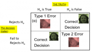
Summing up, when you perform a hypothesis test, there are four possible outcomes depending on the actual truth (or falseness) of the null hypothesis H0 and the decision to reject or not. The outcomes are summarized in the following table:

Table 1. The four possible outcomes in hypothesis testing.

• The decision is not to reject H0 when H0 is true (correct decision).
• The decision is to reject H0 when H0 is true (incorrect decision known as a Type I error ).
• The decision is not to reject H0 when, in fact, H0 is false (incorrect decision known as a Type II error ).
• The decision is to reject H0 when H0 is false ( correct decision ).

Neyman and Pearson coined two terms to describe the probability of these two types of errors in the long run:

• P(Type I error) = αalpha
• P(Type II error) = βbeta

That is, if we set αalpha to .05, then in the long run we should make a Type I error 5% of the time. The 𝞪 (alpha) , is associated with the p-value for the level of significance. Again it’s common to set αalpha as .05. In fact, when the null hypothesis is true and α is .05, we will mistakenly reject the null hypothesis 5% of the time. (This is why α is sometimes referred to as the “Type I error rate.”) In principle, it is possible to reduce the chance of a Type I error by setting α to something less than .05. Setting it to .01, for example, would mean that if the null hypothesis is true, then there is only a 1% chance of mistakenly rejecting it. But making it harder to reject true null hypotheses also makes it harder to reject false ones and therefore increases the chance of a Type II error.

In practice, Type II errors occur primarily because the research design lacks adequate statistical power to detect the relationship (e.g., the sample is too small).  Statistical power is the complement of Type II error. We will have more to say about statistical power shortly. The standard value for an acceptable level of β (beta) is .2 – that is, we are willing to accept that 20% of the time we will fail to detect a true effect when it truly exists. It is possible to reduce the chance of a Type II error by setting α to something greater than .05 (e.g., .10). But making it easier to reject false null hypotheses also makes it easier to reject true ones and therefore increases the chance of a Type I error. This provides some insight into why the convention is to set α to .05. There is some agreement among researchers that level of α keeps the rates of both Type I and Type II errors at acceptable levels.

The possibility of committing Type I and Type II errors has several important implications for interpreting the results of our own and others’ research. One is that we should be cautious about interpreting the results of any individual study because there is a chance that it reflects a Type I or Type II error. This is why researchers consider it important to replicate their studies. Each time researchers replicate a study and find a similar result, they rightly become more confident that the result represents a real phenomenon and not just a Type I or Type II error.

Test Statistic Assumptions

Last consideration we will revisit with each test statistic (e.g., t-test, z-test and ANOVA) in the coming chapters.  There are four main assumptions. These assumptions are often taken for granted in using prescribed data for the course.  In the real world, these assumptions would need to be examined, often tested using statistical software.

• Assumption of random sampling. A sample is random when each person (or animal) point in your population has an equal chance of being included in the sample; therefore selection of any individual happens by chance, rather than by choice. This reduces the chance that differences in materials, characteristics or conditions may bias results. Remember that random samples are more likely to be representative of the population so researchers can be more confident interpreting the results. Note: there is no test that statistical software can perform which assures random sampling has occurred but following good sampling techniques helps to ensure your samples are random.
• Assumption of Independence. Statistical independence is a critical assumption for many statistical tests including the 2-sample t-test and ANOVA. It is assumed that observations are independent of each other often but often this assumption. Is not met. Independence means the value of one observation does not influence or affect the value of other observations. Independent data items are not connected with one another in any way (unless you account for it in your study). Even the smallest dependence in your data can turn into heavily biased results (which may be undetectable) if you violate this assumption. Note: there is no test statistical software can perform that assures independence of the data because this should be addressed during the research planning phase. Using a non-parametric test is often recommended if a researcher is concerned this assumption has been violated.
• Assumption of Normality. Normality assumes that the continuous variables (dependent variable) used in the analysis are normally distributed. Normal distributions are symmetric around the center (the mean) and form a bell-shaped distribution. Normality is violated when sample data are skewed. With large enough sample sizes (n > 30) the violation of the normality assumption should not cause major problems (remember the central limit theorem) but there is a feature in most statistical software that can alert researchers to an assumption violation.
• Assumption of Equal Variance. Variance refers to the spread or of scores from the mean. Many statistical tests assume that although different samples can come from populations with different means, they have the same variance. Equality of variance (i.e., homogeneity of variance) is violated when variances across different groups or samples are significantly different. Note: there is a feature in most statistical software to test for this.

We will use 4 main steps for hypothesis testing:

• Usually the hypotheses concern population parameters and predict the characteristics that a sample should have
• Null: Null hypothesis (H0) states that there is no difference, no effect or no change between population means and sample means. There is no difference.
• Alternative: Alternative hypothesis (H1 or HA) states that there is a difference or a change between the population and sample. It is the opposite of the null hypothesis.
• Set criteria for a decision. In this step we must determine the boundary of our distribution at which the null hypothesis will be rejected. Researchers usually use either a 5% (.05) cutoff or 1% (.01) critical boundary. Recall from our earlier story about Ronald Fisher that the lower the probability the more confident the was that the Tea Lady was not guessing.  We will apply this to z in the next chapter.
• Compare sample and population to decide if the hypothesis has support
• When a researcher uses hypothesis testing, the individual is making a decision about whether the data collected is sufficient to state that the population parameters are significantly different.

Further considerations

The probability value is the probability of a result as extreme or more extreme given that the null hypothesis is true. It is the probability of the data given the null hypothesis. It is not the probability that the null hypothesis is false.

A low probability value indicates that the sample outcome (or one more extreme) would be very unlikely if the null hypothesis were true. We will learn more about assessing effect size later in this unit.

3.  A non-significant outcome means that the data do not conclusively demonstrate that the null hypothesis is false. There is always a chance of error and 4 outcomes associated with hypothesis testing.

• It is important to take into account the assumptions for each test statistic.

Learning objectives

Having read the chapter, you should be able to:

• Identify the components of a hypothesis test, including the parameter of interest, the null and alternative hypotheses, and the test statistic.
• State the hypotheses and identify appropriate critical areas depending on how hypotheses are set up.
• Describe the proper interpretations of a p-value as well as common misinterpretations.
• Distinguish between the two types of error in hypothesis testing, and the factors that determine them.
• Describe the main criticisms of null hypothesis statistical testing
• Identify the purpose of effect size and power.

Exercises – Ch. 9

• In your own words, explain what the null hypothesis is.
• What are Type I and Type II Errors?
• Why do we phrase null and alternative hypotheses with population parameters and not sample means?
• If our null hypothesis is “H0: μ = 40”, what are the three possible alternative hypotheses?
• Why do we state our hypotheses and decision criteria before we collect our data?
• When and why do you calculate an effect size?

Answers to Odd- Numbered Exercises – Ch. 9

1. Your answer should include mention of the baseline assumption of no difference between the sample and the population.

3. Alpha is the significance level. It is the criteria we use when decided to reject or fail to reject the null hypothesis, corresponding to a given proportion of the area under the normal distribution and a probability of finding extreme scores assuming the null hypothesis is true.

5. μ > 40; μ < 40; μ ≠ 40

7. We calculate effect size to determine the strength of the finding.  Effect size should always be calculated when the we have rejected the null hypothesis.  Effect size can be calculated for non-significant findings as a possible indicator of Type II error.

Introduction to Statistics for Psychology Copyright © 2021 by Alisa Beyer is licensed under a Creative Commons Attribution-NonCommercial-ShareAlike 4.0 International License , except where otherwise noted.

Share This Book

Calcworkshop

Hypothesis Testing w/ 21 Step-by-Step Examples!

// Last Updated: October 9, 2020 - Watch Video //

In statistical testing, also referred to as hypothesis testing, our goal is to show the credibility of a claim regarding the population.

Jenn, Founder Calcworkshop ® , 15+ Years Experience (Licensed & Certified Teacher)

What Is Hypothesis Testing

Now it would be unreasonable to assume that we can test the entire population to determine the feasibility of every claim one might have.

Thus, we need a way to conclude an assumption is true or false by taking an appropriate sample and calculating a relevant statistic.

And knowing that we must expect that there will be some variation between the sample statistic that is calculated and the true population parameter, leads us to the understanding of statistical inferences (hypotheses).

Hypothesis Testing Steps

First, we must identify the parameter of interest.

Remember that a parameter always points to the population so that it will be either a population mean, population proportion, population slope, or some other population parameter.

Types of Hypothesis Tests

Then we will write a declaration of our significance test, which will include a null hypothesis statement and an alternative hypothesis.

The null hypothesis is the expected value of the population parameter, similar to the status quo, whereas the alternative hypothesis is a statement of negation of the null hypothesis as discussed by Penn State .

Next, we will calculate the desired test statistic from our random sample. This test statistic is a numerical quantity that measures the difference between the observed value and the expected value, divided by the standard error, which is the sample standard deviation.

Then we will compare this test statistic with a specified level of significance (alpha), just like we did with confidence intervals.

If the probability of yielding the sample statistic is as extreme or more extreme is smaller than our significance level, then we declare the sample statistic to be significant and reject the null hypothesis in favor of the alternative. In other words, if the probability is inside our shaded critical region then it is considered more extreme; thus, rejecting the hypothesis. But if it is outside the critical region, we will fail to reject our claim in favor of the alternative.

Null and Alternative Hypothesis

Additionally, we will also learn how to determine whether our study calls for a one or two-tailed test.

Type 1 And Type 2 Errors

Now, with all inferences and tests of significance, there is always room for error. A Type I error occurs if we reject the null hypothesis, when in actuality, the null hypothesis is true. Similarly, if we fail to reject the null hypothesis when, in reality, the null hypothesis is false, this is considered a Type II error .

Type 1 Vs. Type 2 Error

Imagine you are in a court of law, where a defendant is presumed innocent until proven guilty. What possible errors could a jury make regarding the outcome of the trial?

First, let’s state the following:

• The Null Hypothesis: The defendant is innocent.
• The Alternative Hypothesis: the defendant is guilty.

Now, a Type I Error would happen if the jury rejects the null hypothesis as false when, in reality, the null hypothesis is true. In other words, the jury finds the defendant guilty of a crime they didn’t commit.

And a Type II Error is when a jury accepts the null hypothesis as true when, in reality, the null hypothesis is false. Meaning, the defendant is found innocent of a crime they did commit.

Let’s look at an example where we put all of these ideas together.

Worked Example

Imagine we have a textile manufacturer investigating a new yarn, which claims it has a thread elongation of 12 kilograms with a standard deviation of 0.5 kilograms.

Using a random sample of 4 specimens, the manufacturer wishes to test the claim that the mean thread elongation is less than 12 kilograms.

Write a hypothesis statement for this scenario and using a normal distribution, find the Type 1 error if the sample mean is less than 11.5 kilograms.

Type 1 Error — Example

As we can see, from the example above, the likelihood of a type I error, where the manufacturer rejects the null hypothesis when the null hypothesis is actually true, is approximately 0.023 or 2.3% likely.

Together, we will look at these two types of error and how they affect decision-making and begin to explore the notion of a probability value and how it helps us determine the validity or falsity of our claim.

Hypothesis Testing – Lesson & Examples (Video)

1 hr 17 min

• Introduction to Video: Statistical Hypotheses
• 00:00:38 – Overview of Hypothesis Testing and determining a correctly stated hypothesis testing problem (Examples #1-7)
• Exclusive Content for Members Only
• 00:14:34 – State the Null Hypothesis and the Alternative Hypothesis for each scenario (Examples #8-12)
• 00:25:46 – Hypothesis Testing Steps and Overview of Type I and Type II errors (Examples #13-14)
• 00:40:32 – Describe a Type 1 and Type 2 error (Examples #15-16)
• 00:46:32 – Overview of p-value and Tails of the Hypothesis Test
• 00:55:55 – Find the probability of a Type I and Type II error (Example #17)
• 01:06:08 – Identify null hypothesis, alternative hypothesis, and state whether the scenario is a one-tail or two-tailed test (Examples #18-21)
• Practice Problems with Step-by-Step Solutions
• Chapter Tests with Video Solutions

Get access to all the courses and over 450 HD videos with your subscription

Monthly and Yearly Plans Available

Get My Subscription Now

Still wondering if CalcWorkshop is right for you? Take a Tour and find out how a membership can take the struggle out of learning math.

Hypothesis Testing

Hypothesis testing is a tool for making statistical inferences about the population data. It is an analysis tool that tests assumptions and determines how likely something is within a given standard of accuracy. Hypothesis testing provides a way to verify whether the results of an experiment are valid.

A null hypothesis and an alternative hypothesis are set up before performing the hypothesis testing. This helps to arrive at a conclusion regarding the sample obtained from the population. In this article, we will learn more about hypothesis testing, its types, steps to perform the testing, and associated examples.

What is Hypothesis Testing in Statistics?

Hypothesis testing uses sample data from the population to draw useful conclusions regarding the population probability distribution . It tests an assumption made about the data using different types of hypothesis testing methodologies. The hypothesis testing results in either rejecting or not rejecting the null hypothesis.

Hypothesis Testing Definition

Hypothesis testing can be defined as a statistical tool that is used to identify if the results of an experiment are meaningful or not. It involves setting up a null hypothesis and an alternative hypothesis. These two hypotheses will always be mutually exclusive. This means that if the null hypothesis is true then the alternative hypothesis is false and vice versa. An example of hypothesis testing is setting up a test to check if a new medicine works on a disease in a more efficient manner.

Null Hypothesis

The null hypothesis is a concise mathematical statement that is used to indicate that there is no difference between two possibilities. In other words, there is no difference between certain characteristics of data. This hypothesis assumes that the outcomes of an experiment are based on chance alone. It is denoted as \(H_{0}\). Hypothesis testing is used to conclude if the null hypothesis can be rejected or not. Suppose an experiment is conducted to check if girls are shorter than boys at the age of 5. The null hypothesis will say that they are the same height.

Alternative Hypothesis

The alternative hypothesis is an alternative to the null hypothesis. It is used to show that the observations of an experiment are due to some real effect. It indicates that there is a statistical significance between two possible outcomes and can be denoted as \(H_{1}\) or \(H_{a}\). For the above-mentioned example, the alternative hypothesis would be that girls are shorter than boys at the age of 5.

Hypothesis Testing P Value

In hypothesis testing, the p value is used to indicate whether the results obtained after conducting a test are statistically significant or not. It also indicates the probability of making an error in rejecting or not rejecting the null hypothesis.This value is always a number between 0 and 1. The p value is compared to an alpha level, \(\alpha\) or significance level. The alpha level can be defined as the acceptable risk of incorrectly rejecting the null hypothesis. The alpha level is usually chosen between 1% to 5%.

Hypothesis Testing Critical region

All sets of values that lead to rejecting the null hypothesis lie in the critical region. Furthermore, the value that separates the critical region from the non-critical region is known as the critical value.

Hypothesis Testing Formula

Depending upon the type of data available and the size, different types of hypothesis testing are used to determine whether the null hypothesis can be rejected or not. The hypothesis testing formula for some important test statistics are given below:

• z = \(\frac{\overline{x}-\mu}{\frac{\sigma}{\sqrt{n}}}\). \(\overline{x}\) is the sample mean, \(\mu\) is the population mean, \(\sigma\) is the population standard deviation and n is the size of the sample.
• t = \(\frac{\overline{x}-\mu}{\frac{s}{\sqrt{n}}}\). s is the sample standard deviation.
• \(\chi ^{2} = \sum \frac{(O_{i}-E_{i})^{2}}{E_{i}}\). \(O_{i}\) is the observed value and \(E_{i}\) is the expected value.

We will learn more about these test statistics in the upcoming section.

Types of Hypothesis Testing

Selecting the correct test for performing hypothesis testing can be confusing. These tests are used to determine a test statistic on the basis of which the null hypothesis can either be rejected or not rejected. Some of the important tests used for hypothesis testing are given below.

Hypothesis Testing Z Test

A z test is a way of hypothesis testing that is used for a large sample size (n ≥ 30). It is used to determine whether there is a difference between the population mean and the sample mean when the population standard deviation is known. It can also be used to compare the mean of two samples. It is used to compute the z test statistic. The formulas are given as follows:

• One sample: z = \(\frac{\overline{x}-\mu}{\frac{\sigma}{\sqrt{n}}}\).
• Two samples: z = \(\frac{(\overline{x_{1}}-\overline{x_{2}})-(\mu_{1}-\mu_{2})}{\sqrt{\frac{\sigma_{1}^{2}}{n_{1}}+\frac{\sigma_{2}^{2}}{n_{2}}}}\).

Hypothesis Testing t Test

The t test is another method of hypothesis testing that is used for a small sample size (n < 30). It is also used to compare the sample mean and population mean. However, the population standard deviation is not known. Instead, the sample standard deviation is known. The mean of two samples can also be compared using the t test.

• One sample: t = \(\frac{\overline{x}-\mu}{\frac{s}{\sqrt{n}}}\).
• Two samples: t = \(\frac{(\overline{x_{1}}-\overline{x_{2}})-(\mu_{1}-\mu_{2})}{\sqrt{\frac{s_{1}^{2}}{n_{1}}+\frac{s_{2}^{2}}{n_{2}}}}\).

Hypothesis Testing Chi Square

The Chi square test is a hypothesis testing method that is used to check whether the variables in a population are independent or not. It is used when the test statistic is chi-squared distributed.

One Tailed Hypothesis Testing

One tailed hypothesis testing is done when the rejection region is only in one direction. It can also be known as directional hypothesis testing because the effects can be tested in one direction only. This type of testing is further classified into the right tailed test and left tailed test.

Right Tailed Hypothesis Testing

The right tail test is also known as the upper tail test. This test is used to check whether the population parameter is greater than some value. The null and alternative hypotheses for this test are given as follows:

\(H_{0}\): The population parameter is ≤ some value

\(H_{1}\): The population parameter is > some value.

If the test statistic has a greater value than the critical value then the null hypothesis is rejected

Left Tailed Hypothesis Testing

The left tail test is also known as the lower tail test. It is used to check whether the population parameter is less than some value. The hypotheses for this hypothesis testing can be written as follows:

\(H_{0}\): The population parameter is ≥ some value

\(H_{1}\): The population parameter is < some value.

The null hypothesis is rejected if the test statistic has a value lesser than the critical value.

Two Tailed Hypothesis Testing

In this hypothesis testing method, the critical region lies on both sides of the sampling distribution. It is also known as a non - directional hypothesis testing method. The two-tailed test is used when it needs to be determined if the population parameter is assumed to be different than some value. The hypotheses can be set up as follows:

\(H_{0}\): the population parameter = some value

\(H_{1}\): the population parameter ≠ some value

The null hypothesis is rejected if the test statistic has a value that is not equal to the critical value.

Hypothesis Testing Steps

Hypothesis testing can be easily performed in five simple steps. The most important step is to correctly set up the hypotheses and identify the right method for hypothesis testing. The basic steps to perform hypothesis testing are as follows:

• Step 1: Set up the null hypothesis by correctly identifying whether it is the left-tailed, right-tailed, or two-tailed hypothesis testing.
• Step 2: Set up the alternative hypothesis.
• Step 3: Choose the correct significance level, \(\alpha\), and find the critical value.
• Step 4: Calculate the correct test statistic (z, t or \(\chi\)) and p-value.
• Step 5: Compare the test statistic with the critical value or compare the p-value with \(\alpha\) to arrive at a conclusion. In other words, decide if the null hypothesis is to be rejected or not.

Hypothesis Testing Example

The best way to solve a problem on hypothesis testing is by applying the 5 steps mentioned in the previous section. Suppose a researcher claims that the mean average weight of men is greater than 100kgs with a standard deviation of 15kgs. 30 men are chosen with an average weight of 112.5 Kgs. Using hypothesis testing, check if there is enough evidence to support the researcher's claim. The confidence interval is given as 95%.

Step 1: This is an example of a right-tailed test. Set up the null hypothesis as \(H_{0}\): \(\mu\) = 100.

Step 2: The alternative hypothesis is given by \(H_{1}\): \(\mu\) > 100.

Step 3: As this is a one-tailed test, \(\alpha\) = 100% - 95% = 5%. This can be used to determine the critical value.

1 - \(\alpha\) = 1 - 0.05 = 0.95

0.95 gives the required area under the curve. Now using a normal distribution table, the area 0.95 is at z = 1.645. A similar process can be followed for a t-test. The only additional requirement is to calculate the degrees of freedom given by n - 1.

Step 4: Calculate the z test statistic. This is because the sample size is 30. Furthermore, the sample and population means are known along with the standard deviation.

z = \(\frac{\overline{x}-\mu}{\frac{\sigma}{\sqrt{n}}}\).

\(\mu\) = 100, \(\overline{x}\) = 112.5, n = 30, \(\sigma\) = 15

z = \(\frac{112.5-100}{\frac{15}{\sqrt{30}}}\) = 4.56

Step 5: Conclusion. As 4.56 > 1.645 thus, the null hypothesis can be rejected.

Hypothesis Testing and Confidence Intervals

Confidence intervals form an important part of hypothesis testing. This is because the alpha level can be determined from a given confidence interval. Suppose a confidence interval is given as 95%. Subtract the confidence interval from 100%. This gives 100 - 95 = 5% or 0.05. This is the alpha value of a one-tailed hypothesis testing. To obtain the alpha value for a two-tailed hypothesis testing, divide this value by 2. This gives 0.05 / 2 = 0.025.

Related Articles:

• Probability and Statistics
• Data Handling

Important Notes on Hypothesis Testing

• Hypothesis testing is a technique that is used to verify whether the results of an experiment are statistically significant.
• It involves the setting up of a null hypothesis and an alternate hypothesis.
• There are three types of tests that can be conducted under hypothesis testing - z test, t test, and chi square test.
• Hypothesis testing can be classified as right tail, left tail, and two tail tests.

Examples on Hypothesis Testing

• Example 1: The average weight of a dumbbell in a gym is 90lbs. However, a physical trainer believes that the average weight might be higher. A random sample of 5 dumbbells with an average weight of 110lbs and a standard deviation of 18lbs. Using hypothesis testing check if the physical trainer's claim can be supported for a 95% confidence level. Solution: As the sample size is lesser than 30, the t-test is used. \(H_{0}\): \(\mu\) = 90, \(H_{1}\): \(\mu\) > 90 \(\overline{x}\) = 110, \(\mu\) = 90, n = 5, s = 18. \(\alpha\) = 0.05 Using the t-distribution table, the critical value is 2.132 t = \(\frac{\overline{x}-\mu}{\frac{s}{\sqrt{n}}}\) t = 2.484 As 2.484 > 2.132, the null hypothesis is rejected. Answer: The average weight of the dumbbells may be greater than 90lbs
• Example 2: The average score on a test is 80 with a standard deviation of 10. With a new teaching curriculum introduced it is believed that this score will change. On random testing, the score of 38 students, the mean was found to be 88. With a 0.05 significance level, is there any evidence to support this claim? Solution: This is an example of two-tail hypothesis testing. The z test will be used. \(H_{0}\): \(\mu\) = 80, \(H_{1}\): \(\mu\) ≠ 80 \(\overline{x}\) = 88, \(\mu\) = 80, n = 36, \(\sigma\) = 10. \(\alpha\) = 0.05 / 2 = 0.025 The critical value using the normal distribution table is 1.96 z = \(\frac{\overline{x}-\mu}{\frac{\sigma}{\sqrt{n}}}\) z = \(\frac{88-80}{\frac{10}{\sqrt{36}}}\) = 4.8 As 4.8 > 1.96, the null hypothesis is rejected. Answer: There is a difference in the scores after the new curriculum was introduced.
• Example 3: The average score of a class is 90. However, a teacher believes that the average score might be lower. The scores of 6 students were randomly measured. The mean was 82 with a standard deviation of 18. With a 0.05 significance level use hypothesis testing to check if this claim is true. Solution: The t test will be used. \(H_{0}\): \(\mu\) = 90, \(H_{1}\): \(\mu\) < 90 \(\overline{x}\) = 110, \(\mu\) = 90, n = 6, s = 18 The critical value from the t table is -2.015 t = \(\frac{\overline{x}-\mu}{\frac{s}{\sqrt{n}}}\) t = \(\frac{82-90}{\frac{18}{\sqrt{6}}}\) t = -1.088 As -1.088 > -2.015, we fail to reject the null hypothesis. Answer: There is not enough evidence to support the claim.

go to slide go to slide go to slide

Book a Free Trial Class

FAQs on Hypothesis Testing

What is hypothesis testing.

Hypothesis testing in statistics is a tool that is used to make inferences about the population data. It is also used to check if the results of an experiment are valid.

What is the z Test in Hypothesis Testing?

The z test in hypothesis testing is used to find the z test statistic for normally distributed data . The z test is used when the standard deviation of the population is known and the sample size is greater than or equal to 30.

What is the t Test in Hypothesis Testing?

The t test in hypothesis testing is used when the data follows a student t distribution . It is used when the sample size is less than 30 and standard deviation of the population is not known.

What is the formula for z test in Hypothesis Testing?

The formula for a one sample z test in hypothesis testing is z = \(\frac{\overline{x}-\mu}{\frac{\sigma}{\sqrt{n}}}\) and for two samples is z = \(\frac{(\overline{x_{1}}-\overline{x_{2}})-(\mu_{1}-\mu_{2})}{\sqrt{\frac{\sigma_{1}^{2}}{n_{1}}+\frac{\sigma_{2}^{2}}{n_{2}}}}\).

What is the p Value in Hypothesis Testing?

The p value helps to determine if the test results are statistically significant or not. In hypothesis testing, the null hypothesis can either be rejected or not rejected based on the comparison between the p value and the alpha level.

What is One Tail Hypothesis Testing?

When the rejection region is only on one side of the distribution curve then it is known as one tail hypothesis testing. The right tail test and the left tail test are two types of directional hypothesis testing.

What is the Alpha Level in Two Tail Hypothesis Testing?

To get the alpha level in a two tail hypothesis testing divide \(\alpha\) by 2. This is done as there are two rejection regions in the curve.

Help | Advanced Search

Statistics > Machine Learning

Title: binary hypothesis testing for softmax models and leverage score models.

Abstract: Softmax distributions are widely used in machine learning, including Large Language Models (LLMs) where the attention unit uses softmax distributions. We abstract the attention unit as the softmax model, where given a vector input, the model produces an output drawn from the softmax distribution (which depends on the vector input). We consider the fundamental problem of binary hypothesis testing in the setting of softmax models. That is, given an unknown softmax model, which is known to be one of the two given softmax models, how many queries are needed to determine which one is the truth? We show that the sample complexity is asymptotically $O(\epsilon^{-2})$ where $\epsilon$ is a certain distance between the parameters of the models. Furthermore, we draw analogy between the softmax model and the leverage score model, an important tool for algorithm design in linear algebra and graph theory. The leverage score model, on a high level, is a model which, given vector input, produces an output drawn from a distribution dependent on the input. We obtain similar results for the binary hypothesis testing problem for leverage score models.

Submission history

Access paper:.

• HTML (experimental)
• Other Formats

References & Citations

• Google Scholar
• Semantic Scholar

BibTeX formatted citation

Bibliographic and Citation Tools

Code, data and media associated with this article, recommenders and search tools.

• Institution

arXivLabs: experimental projects with community collaborators

arXivLabs is a framework that allows collaborators to develop and share new arXiv features directly on our website.

Both individuals and organizations that work with arXivLabs have embraced and accepted our values of openness, community, excellence, and user data privacy. arXiv is committed to these values and only works with partners that adhere to them.

Have an idea for a project that will add value for arXiv's community? Learn more about arXivLabs .

• school Campus Bookshelves
• menu_book Bookshelves
• perm_media Learning Objects
• login Login
• how_to_reg Request Instructor Account
• hub Instructor Commons

Margin Size

• Download Page (PDF)
• Download Full Book (PDF)
• Periodic Table
• Physics Constants
• Scientific Calculator
• Reference & Cite
• Tools expand_more
• Readability

selected template will load here

This action is not available.

9.E: Hypothesis Testing with One Sample (Exercises)

• Last updated
• Save as PDF
• Page ID 1146

\( \newcommand{\vecs}[1]{\overset { \scriptstyle \rightharpoonup} {\mathbf{#1}} } \)

\( \newcommand{\vecd}[1]{\overset{-\!-\!\rightharpoonup}{\vphantom{a}\smash {#1}}} \)

\( \newcommand{\id}{\mathrm{id}}\) \( \newcommand{\Span}{\mathrm{span}}\)

( \newcommand{\kernel}{\mathrm{null}\,}\) \( \newcommand{\range}{\mathrm{range}\,}\)

\( \newcommand{\RealPart}{\mathrm{Re}}\) \( \newcommand{\ImaginaryPart}{\mathrm{Im}}\)

\( \newcommand{\Argument}{\mathrm{Arg}}\) \( \newcommand{\norm}[1]{\| #1 \|}\)

\( \newcommand{\inner}[2]{\langle #1, #2 \rangle}\)

\( \newcommand{\Span}{\mathrm{span}}\)

\( \newcommand{\id}{\mathrm{id}}\)

\( \newcommand{\kernel}{\mathrm{null}\,}\)

\( \newcommand{\range}{\mathrm{range}\,}\)

\( \newcommand{\RealPart}{\mathrm{Re}}\)

\( \newcommand{\ImaginaryPart}{\mathrm{Im}}\)

\( \newcommand{\Argument}{\mathrm{Arg}}\)

\( \newcommand{\norm}[1]{\| #1 \|}\)

\( \newcommand{\Span}{\mathrm{span}}\) \( \newcommand{\AA}{\unicode[.8,0]{x212B}}\)

\( \newcommand{\vectorA}[1]{\vec{#1}}      % arrow\)

\( \newcommand{\vectorAt}[1]{\vec{\text{#1}}}      % arrow\)

\( \newcommand{\vectorB}[1]{\overset { \scriptstyle \rightharpoonup} {\mathbf{#1}} } \)

\( \newcommand{\vectorC}[1]{\textbf{#1}} \)

\( \newcommand{\vectorD}[1]{\overrightarrow{#1}} \)

\( \newcommand{\vectorDt}[1]{\overrightarrow{\text{#1}}} \)

\( \newcommand{\vectE}[1]{\overset{-\!-\!\rightharpoonup}{\vphantom{a}\smash{\mathbf {#1}}}} \)

These are homework exercises to accompany the Textmap created for "Introductory Statistics" by OpenStax.

9.1: Introduction

9.2: null and alternative hypotheses.

Some of the following statements refer to the null hypothesis, some to the alternate hypothesis.

State the null hypothesis, \(H_{0}\), and the alternative hypothesis. \(H_{a}\), in terms of the appropriate parameter \((\mu \text{or} p)\).

• The mean number of years Americans work before retiring is 34.
• At most 60% of Americans vote in presidential elections.
• The mean starting salary for San Jose State University graduates is at least $100,000 per year.
• Twenty-nine percent of high school seniors get drunk each month.
• Fewer than 5% of adults ride the bus to work in Los Angeles.
• The mean number of cars a person owns in her lifetime is not more than ten.
• About half of Americans prefer to live away from cities, given the choice.
• Europeans have a mean paid vacation each year of six weeks.
• The chance of developing breast cancer is under 11% for women.
• Private universities' mean tuition cost is more than $20,000 per year.
• \(H_{0}: \mu = 34; H_{a}: \mu \neq 34\)
• \(H_{0}: p \leq 0.60; H_{a}: p > 0.60\)
• \(H_{0}: \mu \geq 100,000; H_{a}: \mu < 100,000\)
• \(H_{0}: p = 0.29; H_{a}: p \neq 0.29\)
• \(H_{0}: p = 0.05; H_{a}: p < 0.05\)
• \(H_{0}: \mu \leq 10; H_{a}: \mu > 10\)
• \(H_{0}: p = 0.50; H_{a}: p \neq 0.50\)
• \(H_{0}: \mu = 6; H_{a}: \mu \neq 6\)
• \(H_{0}: p ≥ 0.11; H_{a}: p < 0.11\)
• \(H_{0}: \mu \leq 20,000; H_{a}: \mu > 20,000\)

Over the past few decades, public health officials have examined the link between weight concerns and teen girls' smoking. Researchers surveyed a group of 273 randomly selected teen girls living in Massachusetts (between 12 and 15 years old). After four years the girls were surveyed again. Sixty-three said they smoked to stay thin. Is there good evidence that more than thirty percent of the teen girls smoke to stay thin? The alternative hypothesis is:

• \(p < 0.30\)
• \(p \leq 0.30\)
• \(p \geq 0.30\)
• \(p > 0.30\)

A statistics instructor believes that fewer than 20% of Evergreen Valley College (EVC) students attended the opening night midnight showing of the latest Harry Potter movie. She surveys 84 of her students and finds that 11 attended the midnight showing. An appropriate alternative hypothesis is:

• \(p = 0.20\)
• \(p > 0.20\)
• \(p < 0.20\)
• \(p \leq 0.20\)

Previously, an organization reported that teenagers spent 4.5 hours per week, on average, on the phone. The organization thinks that, currently, the mean is higher. Fifteen randomly chosen teenagers were asked how many hours per week they spend on the phone. The sample mean was 4.75 hours with a sample standard deviation of 2.0. Conduct a hypothesis test. The null and alternative hypotheses are:

• \(H_{0}: \bar{x} = 4.5, H_{a}: \bar{x} > 4.5\)
• \(H_{0}: \mu \geq 4.5, H_{a}: \mu < 4.5\)
• \(H_{0}: \mu = 4.75, H_{a}: \mu > 4.75\)
• \(H_{0}: \mu = 4.5, H_{a}: \mu > 4.5\)

9.3: Outcomes and the Type I and Type II Errors

State the Type I and Type II errors in complete sentences given the following statements.

• The mean number of cars a person owns in his or her lifetime is not more than ten.
• Private universities mean tuition cost is more than $20,000 per year.
• Type I error: We conclude that the mean is not 34 years, when it really is 34 years. Type II error: We conclude that the mean is 34 years, when in fact it really is not 34 years.
• Type I error: We conclude that more than 60% of Americans vote in presidential elections, when the actual percentage is at most 60%.Type II error: We conclude that at most 60% of Americans vote in presidential elections when, in fact, more than 60% do.
• Type I error: We conclude that the mean starting salary is less than $100,000, when it really is at least $100,000. Type II error: We conclude that the mean starting salary is at least $100,000 when, in fact, it is less than $100,000.
• Type I error: We conclude that the proportion of high school seniors who get drunk each month is not 29%, when it really is 29%. Type II error: We conclude that the proportion of high school seniors who get drunk each month is 29% when, in fact, it is not 29%.
• Type I error: We conclude that fewer than 5% of adults ride the bus to work in Los Angeles, when the percentage that do is really 5% or more. Type II error: We conclude that 5% or more adults ride the bus to work in Los Angeles when, in fact, fewer that 5% do.
• Type I error: We conclude that the mean number of cars a person owns in his or her lifetime is more than 10, when in reality it is not more than 10. Type II error: We conclude that the mean number of cars a person owns in his or her lifetime is not more than 10 when, in fact, it is more than 10.
• Type I error: We conclude that the proportion of Americans who prefer to live away from cities is not about half, though the actual proportion is about half. Type II error: We conclude that the proportion of Americans who prefer to live away from cities is half when, in fact, it is not half.
• Type I error: We conclude that the duration of paid vacations each year for Europeans is not six weeks, when in fact it is six weeks. Type II error: We conclude that the duration of paid vacations each year for Europeans is six weeks when, in fact, it is not.
• Type I error: We conclude that the proportion is less than 11%, when it is really at least 11%. Type II error: We conclude that the proportion of women who develop breast cancer is at least 11%, when in fact it is less than 11%.
• Type I error: We conclude that the average tuition cost at private universities is more than $20,000, though in reality it is at most $20,000. Type II error: We conclude that the average tuition cost at private universities is at most $20,000 when, in fact, it is more than $20,000.

For statements a-j in Exercise 9.109 , answer the following in complete sentences.

• State a consequence of committing a Type I error.
• State a consequence of committing a Type II error.

When a new drug is created, the pharmaceutical company must subject it to testing before receiving the necessary permission from the Food and Drug Administration (FDA) to market the drug. Suppose the null hypothesis is “the drug is unsafe.” What is the Type II Error?

• To conclude the drug is safe when in, fact, it is unsafe.
• Not to conclude the drug is safe when, in fact, it is safe.
• To conclude the drug is safe when, in fact, it is safe.
• Not to conclude the drug is unsafe when, in fact, it is unsafe.

A statistics instructor believes that fewer than 20% of Evergreen Valley College (EVC) students attended the opening midnight showing of the latest Harry Potter movie. She surveys 84 of her students and finds that 11 of them attended the midnight showing. The Type I error is to conclude that the percent of EVC students who attended is ________.

• at least 20%, when in fact, it is less than 20%.
• 20%, when in fact, it is 20%.
• less than 20%, when in fact, it is at least 20%.
• less than 20%, when in fact, it is less than 20%.

It is believed that Lake Tahoe Community College (LTCC) Intermediate Algebra students get less than seven hours of sleep per night, on average. A survey of 22 LTCC Intermediate Algebra students generated a mean of 7.24 hours with a standard deviation of 1.93 hours. At a level of significance of 5%, do LTCC Intermediate Algebra students get less than seven hours of sleep per night, on average?

The Type II error is not to reject that the mean number of hours of sleep LTCC students get per night is at least seven when, in fact, the mean number of hours

• is more than seven hours.
• is at most seven hours.
• is at least seven hours.
• is less than seven hours.

Previously, an organization reported that teenagers spent 4.5 hours per week, on average, on the phone. The organization thinks that, currently, the mean is higher. Fifteen randomly chosen teenagers were asked how many hours per week they spend on the phone. The sample mean was 4.75 hours with a sample standard deviation of 2.0. Conduct a hypothesis test, the Type I error is:

• to conclude that the current mean hours per week is higher than 4.5, when in fact, it is higher
• to conclude that the current mean hours per week is higher than 4.5, when in fact, it is the same
• to conclude that the mean hours per week currently is 4.5, when in fact, it is higher
• to conclude that the mean hours per week currently is no higher than 4.5, when in fact, it is not higher

9.4: Distribution Needed for Hypothesis Testing

It is believed that Lake Tahoe Community College (LTCC) Intermediate Algebra students get less than seven hours of sleep per night, on average. A survey of 22 LTCC Intermediate Algebra students generated a mean of 7.24 hours with a standard deviation of 1.93 hours. At a level of significance of 5%, do LTCC Intermediate Algebra students get less than seven hours of sleep per night, on average? The distribution to be used for this test is \(\bar{X} \sim\) ________________

• \(N\left(7.24, \frac{1.93}{\sqrt{22}}\right)\)
• \(N\left(7.24, 1.93\right)\)

9.5: Rare Events, the Sample, Decision and Conclusion

The National Institute of Mental Health published an article stating that in any one-year period, approximately 9.5 percent of American adults suffer from depression or a depressive illness. Suppose that in a survey of 100 people in a certain town, seven of them suffered from depression or a depressive illness. Conduct a hypothesis test to determine if the true proportion of people in that town suffering from depression or a depressive illness is lower than the percent in the general adult American population.

• Is this a test of one mean or proportion?
• State the null and alternative hypotheses. \(H_{0}\) : ____________________ \(H_{a}\) : ____________________
• Is this a right-tailed, left-tailed, or two-tailed test?
• What symbol represents the random variable for this test?
• In words, define the random variable for this test.
• \(x =\) ________________
• \(n =\) ________________
• \(p′ =\) _____________
• Calculate \(\sigma_{x} =\) __________. Show the formula set-up.
• State the distribution to use for the hypothesis test.
• Find the \(p\text{-value}\).
• Reason for the decision:
• Conclusion (write out in a complete sentence):

9.6: Additional Information and Full Hypothesis Test Examples

For each of the word problems, use a solution sheet to do the hypothesis test. The solution sheet is found in [link] . Please feel free to make copies of the solution sheets. For the online version of the book, it is suggested that you copy the .doc or the .pdf files.

If you are using a Student's \(t\) - distribution for one of the following homework problems, you may assume that the underlying population is normally distributed. (In general, you must first prove that assumption, however.)

A particular brand of tires claims that its deluxe tire averages at least 50,000 miles before it needs to be replaced. From past studies of this tire, the standard deviation is known to be 8,000. A survey of owners of that tire design is conducted. From the 28 tires surveyed, the mean lifespan was 46,500 miles with a standard deviation of 9,800 miles. Using \(\alpha = 0.05\), is the data highly inconsistent with the claim?

• \(H_{0}: \mu \geq 50,000\)
• \(H_{a}: \mu < 50,000\)
• Let \(\bar{X} =\) the average lifespan of a brand of tires.
• normal distribution
• \(z = -2.315\)
• \(p\text{-value} = 0.0103\)
• Check student’s solution.
• alpha: 0.05
• Decision: Reject the null hypothesis.
• Reason for decision: The \(p\text{-value}\) is less than 0.05.
• Conclusion: There is sufficient evidence to conclude that the mean lifespan of the tires is less than 50,000 miles.
• \((43,537, 49,463)\)

From generation to generation, the mean age when smokers first start to smoke varies. However, the standard deviation of that age remains constant of around 2.1 years. A survey of 40 smokers of this generation was done to see if the mean starting age is at least 19. The sample mean was 18.1 with a sample standard deviation of 1.3. Do the data support the claim at the 5% level?

The cost of a daily newspaper varies from city to city. However, the variation among prices remains steady with a standard deviation of 20¢. A study was done to test the claim that the mean cost of a daily newspaper is $1.00. Twelve costs yield a mean cost of 95¢ with a standard deviation of 18¢. Do the data support the claim at the 1% level?

• \(H_{0}: \mu = $1.00\)
• \(H_{a}: \mu \neq $1.00\)
• Let \(\bar{X} =\) the average cost of a daily newspaper.
• \(z = –0.866\)
• \(p\text{-value} = 0.3865\)
• \(\alpha: 0.01\)
• Decision: Do not reject the null hypothesis.
• Reason for decision: The \(p\text{-value}\) is greater than 0.01.
• Conclusion: There is sufficient evidence to support the claim that the mean cost of daily papers is $1. The mean cost could be $1.
• \(($0.84, $1.06)\)

An article in the San Jose Mercury News stated that students in the California state university system take 4.5 years, on average, to finish their undergraduate degrees. Suppose you believe that the mean time is longer. You conduct a survey of 49 students and obtain a sample mean of 5.1 with a sample standard deviation of 1.2. Do the data support your claim at the 1% level?

The mean number of sick days an employee takes per year is believed to be about ten. Members of a personnel department do not believe this figure. They randomly survey eight employees. The number of sick days they took for the past year are as follows: 12; 4; 15; 3; 11; 8; 6; 8. Let \(x =\) the number of sick days they took for the past year. Should the personnel team believe that the mean number is ten?

• \(H_{0}: \mu = 10\)
• \(H_{a}: \mu \neq 10\)
• Let \(\bar{X}\) the mean number of sick days an employee takes per year.
• Student’s t -distribution
• \(t = –1.12\)
• \(p\text{-value} = 0.300\)
• \(\alpha: 0.05\)
• Reason for decision: The \(p\text{-value}\) is greater than 0.05.
• Conclusion: At the 5% significance level, there is insufficient evidence to conclude that the mean number of sick days is not ten.
• \((4.9443, 11.806)\)

In 1955, Life Magazine reported that the 25 year-old mother of three worked, on average, an 80 hour week. Recently, many groups have been studying whether or not the women's movement has, in fact, resulted in an increase in the average work week for women (combining employment and at-home work). Suppose a study was done to determine if the mean work week has increased. 81 women were surveyed with the following results. The sample mean was 83; the sample standard deviation was ten. Does it appear that the mean work week has increased for women at the 5% level?

Your statistics instructor claims that 60 percent of the students who take her Elementary Statistics class go through life feeling more enriched. For some reason that she can't quite figure out, most people don't believe her. You decide to check this out on your own. You randomly survey 64 of her past Elementary Statistics students and find that 34 feel more enriched as a result of her class. Now, what do you think?

• \(H_{0}: p \geq 0.6\)
• \(H_{a}: p < 0.6\)
• Let \(P′ =\) the proportion of students who feel more enriched as a result of taking Elementary Statistics.
• normal for a single proportion
• \(p\text{-value} = 0.1308\)
• Conclusion: There is insufficient evidence to conclude that less than 60 percent of her students feel more enriched.

The “plus-4s” confidence interval is \((0.411, 0.648)\)

A Nissan Motor Corporation advertisement read, “The average man’s I.Q. is 107. The average brown trout’s I.Q. is 4. So why can’t man catch brown trout?” Suppose you believe that the brown trout’s mean I.Q. is greater than four. You catch 12 brown trout. A fish psychologist determines the I.Q.s as follows: 5; 4; 7; 3; 6; 4; 5; 3; 6; 3; 8; 5. Conduct a hypothesis test of your belief.

Refer to Exercise 9.119 . Conduct a hypothesis test to see if your decision and conclusion would change if your belief were that the brown trout’s mean I.Q. is not four.

• \(H_{0}: \mu = 4\)
• \(H_{a}: \mu \neq 4\)
• Let \(\bar{X}\) the average I.Q. of a set of brown trout.
• two-tailed Student's t-test
• \(t = 1.95\)
• \(p\text{-value} = 0.076\)
• Reason for decision: The \(p\text{-value}\) is greater than 0.05
• Conclusion: There is insufficient evidence to conclude that the average IQ of brown trout is not four.
• \((3.8865,5.9468)\)

According to an article in Newsweek , the natural ratio of girls to boys is 100:105. In China, the birth ratio is 100: 114 (46.7% girls). Suppose you don’t believe the reported figures of the percent of girls born in China. You conduct a study. In this study, you count the number of girls and boys born in 150 randomly chosen recent births. There are 60 girls and 90 boys born of the 150. Based on your study, do you believe that the percent of girls born in China is 46.7?

A poll done for Newsweek found that 13% of Americans have seen or sensed the presence of an angel. A contingent doubts that the percent is really that high. It conducts its own survey. Out of 76 Americans surveyed, only two had seen or sensed the presence of an angel. As a result of the contingent’s survey, would you agree with the Newsweek poll? In complete sentences, also give three reasons why the two polls might give different results.

• \(H_{a}: p < 0.13\)
• Let \(P′ =\) the proportion of Americans who have seen or sensed angels
• –2.688
• \(p\text{-value} = 0.0036\)
• Reason for decision: The \(p\text{-value}\)e is less than 0.05.
• Conclusion: There is sufficient evidence to conclude that the percentage of Americans who have seen or sensed an angel is less than 13%.

The“plus-4s” confidence interval is (0.0022, 0.0978)

The mean work week for engineers in a start-up company is believed to be about 60 hours. A newly hired engineer hopes that it’s shorter. She asks ten engineering friends in start-ups for the lengths of their mean work weeks. Based on the results that follow, should she count on the mean work week to be shorter than 60 hours?

Data (length of mean work week): 70; 45; 55; 60; 65; 55; 55; 60; 50; 55.

Use the “Lap time” data for Lap 4 (see [link] ) to test the claim that Terri finishes Lap 4, on average, in less than 129 seconds. Use all twenty races given.

• \(H_{0}: \mu \geq 129\)
• \(H_{a}: \mu < 129\)
• Let \(\bar{X} =\) the average time in seconds that Terri finishes Lap 4.
• Student's t -distribution
• \(t = 1.209\)
• Conclusion: There is insufficient evidence to conclude that Terri’s mean lap time is less than 129 seconds.
• \((128.63, 130.37)\)

Use the “Initial Public Offering” data (see [link] ) to test the claim that the mean offer price was $18 per share. Do not use all the data. Use your random number generator to randomly survey 15 prices.

The following questions were written by past students. They are excellent problems!

"Asian Family Reunion," by Chau Nguyen

Every two years it comes around.

We all get together from different towns.

In my honest opinion,

It's not a typical family reunion.

Not forty, or fifty, or sixty,

But how about seventy companions!

The kids would play, scream, and shout

One minute they're happy, another they'll pout.

The teenagers would look, stare, and compare

From how they look to what they wear.

The men would chat about their business

That they make more, but never less.

Money is always their subject

And there's always talk of more new projects.

The women get tired from all of the chats

They head to the kitchen to set out the mats.

Some would sit and some would stand

Eating and talking with plates in their hands.

Then come the games and the songs

And suddenly, everyone gets along!

With all that laughter, it's sad to say

That it always ends in the same old way.

They hug and kiss and say "good-bye"

And then they all begin to cry!

I say that 60 percent shed their tears

But my mom counted 35 people this year.

She said that boys and men will always have their pride,

So we won't ever see them cry.

I myself don't think she's correct,

So could you please try this problem to see if you object?

• \(H_{0}: p = 0.60\)
• \(H_{a}: p < 0.60\)
• Let \(P′ =\) the proportion of family members who shed tears at a reunion.
• –1.71
• Reason for decision: \(p\text{-value} < \alpha\)
• Conclusion: At the 5% significance level, there is sufficient evidence to conclude that the proportion of family members who shed tears at a reunion is less than 0.60. However, the test is weak because the \(p\text{-value}\) and alpha are quite close, so other tests should be done.
• We are 95% confident that between 38.29% and 61.71% of family members will shed tears at a family reunion. \((0.3829, 0.6171)\). The“plus-4s” confidence interval (see chapter 8) is \((0.3861, 0.6139)\)

Note that here the “large-sample” \(1 - \text{PropZTest}\) provides the approximate \(p\text{-value}\) of 0.0438. Whenever a \(p\text{-value}\) based on a normal approximation is close to the level of significance, the exact \(p\text{-value}\) based on binomial probabilities should be calculated whenever possible. This is beyond the scope of this course.

"The Problem with Angels," by Cyndy Dowling

Although this problem is wholly mine,

The catalyst came from the magazine, Time.

On the magazine cover I did find

The realm of angels tickling my mind.

Inside, 69% I found to be

In angels, Americans do believe.

Then, it was time to rise to the task,

Ninety-five high school and college students I did ask.

Viewing all as one group,

Random sampling to get the scoop.

So, I asked each to be true,

"Do you believe in angels?" Tell me, do!

Hypothesizing at the start,

Totally believing in my heart

That the proportion who said yes

Would be equal on this test.

Lo and behold, seventy-three did arrive,

Out of the sample of ninety-five.

Now your job has just begun,

Solve this problem and have some fun.

"Blowing Bubbles," by Sondra Prull

Studying stats just made me tense,

I had to find some sane defense.

Some light and lifting simple play

To float my math anxiety away.

Blowing bubbles lifts me high

Takes my troubles to the sky.

POIK! They're gone, with all my stress

Bubble therapy is the best.

The label said each time I blew

The average number of bubbles would be at least 22.

I blew and blew and this I found

From 64 blows, they all are round!

But the number of bubbles in 64 blows

Varied widely, this I know.

20 per blow became the mean

They deviated by 6, and not 16.

From counting bubbles, I sure did relax

But now I give to you your task.

Was 22 a reasonable guess?

Find the answer and pass this test!

• \(H_{0}: \mu \geq 22\)
• \(H_{a}: \mu < 22\)
• Let \(\bar{X} =\) the mean number of bubbles per blow.
• –2.667
• \(p\text{-value} = 0.00486\)
• Conclusion: There is sufficient evidence to conclude that the mean number of bubbles per blow is less than 22.
• \((18.501, 21.499)\)

"Dalmatian Darnation," by Kathy Sparling

A greedy dog breeder named Spreckles

Bred puppies with numerous freckles

The Dalmatians he sought

Possessed spot upon spot

The more spots, he thought, the more shekels.

His competitors did not agree

That freckles would increase the fee.

They said, “Spots are quite nice

But they don't affect price;

One should breed for improved pedigree.”

The breeders decided to prove

This strategy was a wrong move.

Breeding only for spots

Would wreak havoc, they thought.

His theory they want to disprove.

They proposed a contest to Spreckles

Comparing dog prices to freckles.

In records they looked up

One hundred one pups:

Dalmatians that fetched the most shekels.

They asked Mr. Spreckles to name

An average spot count he'd claim

To bring in big bucks.

Said Spreckles, “Well, shucks,

It's for one hundred one that I aim.”

Said an amateur statistician

Who wanted to help with this mission.

“Twenty-one for the sample

Standard deviation's ample:

They examined one hundred and one

Dalmatians that fetched a good sum.

They counted each spot,

Mark, freckle and dot

And tallied up every one.

Instead of one hundred one spots

They averaged ninety six dots

Can they muzzle Spreckles’

Obsession with freckles

Based on all the dog data they've got?

"Macaroni and Cheese, please!!" by Nedda Misherghi and Rachelle Hall

As a poor starving student I don't have much money to spend for even the bare necessities. So my favorite and main staple food is macaroni and cheese. It's high in taste and low in cost and nutritional value.

One day, as I sat down to determine the meaning of life, I got a serious craving for this, oh, so important, food of my life. So I went down the street to Greatway to get a box of macaroni and cheese, but it was SO expensive! $2.02 !!! Can you believe it? It made me stop and think. The world is changing fast. I had thought that the mean cost of a box (the normal size, not some super-gigantic-family-value-pack) was at most $1, but now I wasn't so sure. However, I was determined to find out. I went to 53 of the closest grocery stores and surveyed the prices of macaroni and cheese. Here are the data I wrote in my notebook:

Price per box of Mac and Cheese:

• 5 stores @ $2.02
• 15 stores @ $0.25
• 3 stores @ $1.29
• 6 stores @ $0.35
• 4 stores @ $2.27
• 7 stores @ $1.50
• 5 stores @ $1.89
• 8 stores @ 0.75.

I could see that the cost varied but I had to sit down to figure out whether or not I was right. If it does turn out that this mouth-watering dish is at most $1, then I'll throw a big cheesy party in our next statistics lab, with enough macaroni and cheese for just me. (After all, as a poor starving student I can't be expected to feed our class of animals!)

• \(H_{0}: \mu \leq 1\)
• \(H_{a}: \mu > 1\)
• Let \(\bar{X} =\) the mean cost in dollars of macaroni and cheese in a certain town.
• Student's \(t\)-distribution
• \(t = 0.340\)
• \(p\text{-value} = 0.36756\)
• Conclusion: The mean cost could be $1, or less. At the 5% significance level, there is insufficient evidence to conclude that the mean price of a box of macaroni and cheese is more than $1.
• \((0.8291, 1.241)\)

"William Shakespeare: The Tragedy of Hamlet, Prince of Denmark," by Jacqueline Ghodsi

THE CHARACTERS (in order of appearance):

• HAMLET, Prince of Denmark and student of Statistics
• POLONIUS, Hamlet’s tutor
• HOROTIO, friend to Hamlet and fellow student

Scene: The great library of the castle, in which Hamlet does his lessons

(The day is fair, but the face of Hamlet is clouded. He paces the large room. His tutor, Polonius, is reprimanding Hamlet regarding the latter’s recent experience. Horatio is seated at the large table at right stage.)

POLONIUS: My Lord, how cans’t thou admit that thou hast seen a ghost! It is but a figment of your imagination!

HAMLET: I beg to differ; I know of a certainty that five-and-seventy in one hundred of us, condemned to the whips and scorns of time as we are, have gazed upon a spirit of health, or goblin damn’d, be their intents wicked or charitable.

POLONIUS If thou doest insist upon thy wretched vision then let me invest your time; be true to thy work and speak to me through the reason of the null and alternate hypotheses. (He turns to Horatio.) Did not Hamlet himself say, “What piece of work is man, how noble in reason, how infinite in faculties? Then let not this foolishness persist. Go, Horatio, make a survey of three-and-sixty and discover what the true proportion be. For my part, I will never succumb to this fantasy, but deem man to be devoid of all reason should thy proposal of at least five-and-seventy in one hundred hold true.

HORATIO (to Hamlet): What should we do, my Lord?

HAMLET: Go to thy purpose, Horatio.

HORATIO: To what end, my Lord?

HAMLET: That you must teach me. But let me conjure you by the rights of our fellowship, by the consonance of our youth, but the obligation of our ever-preserved love, be even and direct with me, whether I am right or no.

(Horatio exits, followed by Polonius, leaving Hamlet to ponder alone.)

(The next day, Hamlet awaits anxiously the presence of his friend, Horatio. Polonius enters and places some books upon the table just a moment before Horatio enters.)

POLONIUS: So, Horatio, what is it thou didst reveal through thy deliberations?

HORATIO: In a random survey, for which purpose thou thyself sent me forth, I did discover that one-and-forty believe fervently that the spirits of the dead walk with us. Before my God, I might not this believe, without the sensible and true avouch of mine own eyes.

POLONIUS: Give thine own thoughts no tongue, Horatio. (Polonius turns to Hamlet.) But look to’t I charge you, my Lord. Come Horatio, let us go together, for this is not our test. (Horatio and Polonius leave together.)

HAMLET: To reject, or not reject, that is the question: whether ‘tis nobler in the mind to suffer the slings and arrows of outrageous statistics, or to take arms against a sea of data, and, by opposing, end them. (Hamlet resignedly attends to his task.)

(Curtain falls)

"Untitled," by Stephen Chen

I've often wondered how software is released and sold to the public. Ironically, I work for a company that sells products with known problems. Unfortunately, most of the problems are difficult to create, which makes them difficult to fix. I usually use the test program X, which tests the product, to try to create a specific problem. When the test program is run to make an error occur, the likelihood of generating an error is 1%.

So, armed with this knowledge, I wrote a new test program Y that will generate the same error that test program X creates, but more often. To find out if my test program is better than the original, so that I can convince the management that I'm right, I ran my test program to find out how often I can generate the same error. When I ran my test program 50 times, I generated the error twice. While this may not seem much better, I think that I can convince the management to use my test program instead of the original test program. Am I right?

• \(H_{0}: p = 0.01\)
• \(H_{a}: p > 0.01\)
• Let \(P′ =\) the proportion of errors generated
• Normal for a single proportion
• Decision: Reject the null hypothesis
• Conclusion: At the 5% significance level, there is sufficient evidence to conclude that the proportion of errors generated is more than 0.01.

The“plus-4s” confidence interval is \((0.004, 0.144)\).

"Japanese Girls’ Names"

by Kumi Furuichi

It used to be very typical for Japanese girls’ names to end with “ko.” (The trend might have started around my grandmothers’ generation and its peak might have been around my mother’s generation.) “Ko” means “child” in Chinese characters. Parents would name their daughters with “ko” attaching to other Chinese characters which have meanings that they want their daughters to become, such as Sachiko—happy child, Yoshiko—a good child, Yasuko—a healthy child, and so on.

However, I noticed recently that only two out of nine of my Japanese girlfriends at this school have names which end with “ko.” More and more, parents seem to have become creative, modernized, and, sometimes, westernized in naming their children.

I have a feeling that, while 70 percent or more of my mother’s generation would have names with “ko” at the end, the proportion has dropped among my peers. I wrote down all my Japanese friends’, ex-classmates’, co-workers, and acquaintances’ names that I could remember. Following are the names. (Some are repeats.) Test to see if the proportion has dropped for this generation.

Ai, Akemi, Akiko, Ayumi, Chiaki, Chie, Eiko, Eri, Eriko, Fumiko, Harumi, Hitomi, Hiroko, Hiroko, Hidemi, Hisako, Hinako, Izumi, Izumi, Junko, Junko, Kana, Kanako, Kanayo, Kayo, Kayoko, Kazumi, Keiko, Keiko, Kei, Kumi, Kumiko, Kyoko, Kyoko, Madoka, Maho, Mai, Maiko, Maki, Miki, Miki, Mikiko, Mina, Minako, Miyako, Momoko, Nana, Naoko, Naoko, Naoko, Noriko, Rieko, Rika, Rika, Rumiko, Rei, Reiko, Reiko, Sachiko, Sachiko, Sachiyo, Saki, Sayaka, Sayoko, Sayuri, Seiko, Shiho, Shizuka, Sumiko, Takako, Takako, Tomoe, Tomoe, Tomoko, Touko, Yasuko, Yasuko, Yasuyo, Yoko, Yoko, Yoko, Yoshiko, Yoshiko, Yoshiko, Yuka, Yuki, Yuki, Yukiko, Yuko, Yuko.

"Phillip’s Wish," by Suzanne Osorio

My nephew likes to play

Chasing the girls makes his day.

He asked his mother

If it is okay

To get his ear pierced.

She said, “No way!”

To poke a hole through your ear,

Is not what I want for you, dear.

He argued his point quite well,

Says even my macho pal, Mel,

Has gotten this done.

It’s all just for fun.

C’mon please, mom, please, what the hell.

Again Phillip complained to his mother,

Saying half his friends (including their brothers)

Are piercing their ears

And they have no fears

He wants to be like the others.

She said, “I think it’s much less.

We must do a hypothesis test.

And if you are right,

I won’t put up a fight.

But, if not, then my case will rest.”

We proceeded to call fifty guys

To see whose prediction would fly.

Nineteen of the fifty

Said piercing was nifty

And earrings they’d occasionally buy.

Then there’s the other thirty-one,

Who said they’d never have this done.

So now this poem’s finished.

Will his hopes be diminished,

Or will my nephew have his fun?

• \(H_{0}: p = 0.50\)
• \(H_{a}: p < 0.50\)
• Let \(P′ =\) the proportion of friends that has a pierced ear.
• –1.70
• \(p\text{-value} = 0.0448\)
• Reason for decision: The \(p\text{-value}\) is less than 0.05. (However, they are very close.)
• Conclusion: There is sufficient evidence to support the claim that less than 50% of his friends have pierced ears.
• Confidence Interval: \((0.245, 0.515)\): The “plus-4s” confidence interval is \((0.259, 0.519)\).

"The Craven," by Mark Salangsang

Once upon a morning dreary

In stats class I was weak and weary.

Pondering over last night’s homework

Whose answers were now on the board

This I did and nothing more.

While I nodded nearly napping

Suddenly, there came a tapping.

As someone gently rapping,

Rapping my head as I snore.

Quoth the teacher, “Sleep no more.”

“In every class you fall asleep,”

The teacher said, his voice was deep.

“So a tally I’ve begun to keep

Of every class you nap and snore.

The percentage being forty-four.”

“My dear teacher I must confess,

While sleeping is what I do best.

The percentage, I think, must be less,

A percentage less than forty-four.”

This I said and nothing more.

“We’ll see,” he said and walked away,

And fifty classes from that day

He counted till the month of May

The classes in which I napped and snored.

The number he found was twenty-four.

At a significance level of 0.05,

Please tell me am I still alive?

Or did my grade just take a dive

Plunging down beneath the floor?

Upon thee I hereby implore.

Toastmasters International cites a report by Gallop Poll that 40% of Americans fear public speaking. A student believes that less than 40% of students at her school fear public speaking. She randomly surveys 361 schoolmates and finds that 135 report they fear public speaking. Conduct a hypothesis test to determine if the percent at her school is less than 40%.

• \(H_{0}: p = 0.40\)
• \(H_{a}: p < 0.40\)
• Let \(P′ =\) the proportion of schoolmates who fear public speaking.
• –1.01
• \(p\text{-value} = 0.1563\)
• Conclusion: There is insufficient evidence to support the claim that less than 40% of students at the school fear public speaking.
• Confidence Interval: \((0.3241, 0.4240)\): The “plus-4s” confidence interval is \((0.3257, 0.4250)\).

Sixty-eight percent of online courses taught at community colleges nationwide were taught by full-time faculty. To test if 68% also represents California’s percent for full-time faculty teaching the online classes, Long Beach City College (LBCC) in California, was randomly selected for comparison. In the same year, 34 of the 44 online courses LBCC offered were taught by full-time faculty. Conduct a hypothesis test to determine if 68% represents California. NOTE: For more accurate results, use more California community colleges and this past year's data.

According to an article in Bloomberg Businessweek , New York City's most recent adult smoking rate is 14%. Suppose that a survey is conducted to determine this year’s rate. Nine out of 70 randomly chosen N.Y. City residents reply that they smoke. Conduct a hypothesis test to determine if the rate is still 14% or if it has decreased.

• \(H_{0}: p = 0.14\)
• \(H_{a}: p < 0.14\)
• Let \(P′ =\) the proportion of NYC residents that smoke.
• –0.2756
• \(p\text{-value} = 0.3914\)
• At the 5% significance level, there is insufficient evidence to conclude that the proportion of NYC residents who smoke is less than 0.14.
• Confidence Interval: \((0.0502, 0.2070)\): The “plus-4s” confidence interval (see chapter 8) is \((0.0676, 0.2297)\).

The mean age of De Anza College students in a previous term was 26.6 years old. An instructor thinks the mean age for online students is older than 26.6. She randomly surveys 56 online students and finds that the sample mean is 29.4 with a standard deviation of 2.1. Conduct a hypothesis test.

Registered nurses earned an average annual salary of $69,110. For that same year, a survey was conducted of 41 California registered nurses to determine if the annual salary is higher than $69,110 for California nurses. The sample average was $71,121 with a sample standard deviation of $7,489. Conduct a hypothesis test.

• \(H_{0}: \mu = 69,110\)
• \(H_{0}: \mu > 69,110\)
• Let \(\bar{X} =\) the mean salary in dollars for California registered nurses.
• \(t = 1.719\)
• \(p\text{-value}: 0.0466\)
• Conclusion: At the 5% significance level, there is sufficient evidence to conclude that the mean salary of California registered nurses exceeds $69,110.
• \(($68,757, $73,485)\)

La Leche League International reports that the mean age of weaning a child from breastfeeding is age four to five worldwide. In America, most nursing mothers wean their children much earlier. Suppose a random survey is conducted of 21 U.S. mothers who recently weaned their children. The mean weaning age was nine months (3/4 year) with a standard deviation of 4 months. Conduct a hypothesis test to determine if the mean weaning age in the U.S. is less than four years old.

Over the past few decades, public health officials have examined the link between weight concerns and teen girls' smoking. Researchers surveyed a group of 273 randomly selected teen girls living in Massachusetts (between 12 and 15 years old). After four years the girls were surveyed again. Sixty-three said they smoked to stay thin. Is there good evidence that more than thirty percent of the teen girls smoke to stay thin?

After conducting the test, your decision and conclusion are

• Reject \(H_{0}\): There is sufficient evidence to conclude that more than 30% of teen girls smoke to stay thin.
• Do not reject \(H_{0}\): There is not sufficient evidence to conclude that less than 30% of teen girls smoke to stay thin.
• Do not reject \(H_{0}\): There is not sufficient evidence to conclude that more than 30% of teen girls smoke to stay thin.
• Reject \(H_{0}\): There is sufficient evidence to conclude that less than 30% of teen girls smoke to stay thin.

A statistics instructor believes that fewer than 20% of Evergreen Valley College (EVC) students attended the opening night midnight showing of the latest Harry Potter movie. She surveys 84 of her students and finds that 11 of them attended the midnight showing.

At a 1% level of significance, an appropriate conclusion is:

• There is insufficient evidence to conclude that the percent of EVC students who attended the midnight showing of Harry Potter is less than 20%.
• There is sufficient evidence to conclude that the percent of EVC students who attended the midnight showing of Harry Potter is more than 20%.
• There is sufficient evidence to conclude that the percent of EVC students who attended the midnight showing of Harry Potter is less than 20%.
• There is insufficient evidence to conclude that the percent of EVC students who attended the midnight showing of Harry Potter is at least 20%.

Previously, an organization reported that teenagers spent 4.5 hours per week, on average, on the phone. The organization thinks that, currently, the mean is higher. Fifteen randomly chosen teenagers were asked how many hours per week they spend on the phone. The sample mean was 4.75 hours with a sample standard deviation of 2.0. Conduct a hypothesis test.

At a significance level of \(a = 0.05\), what is the correct conclusion?

• There is enough evidence to conclude that the mean number of hours is more than 4.75
• There is enough evidence to conclude that the mean number of hours is more than 4.5
• There is not enough evidence to conclude that the mean number of hours is more than 4.5
• There is not enough evidence to conclude that the mean number of hours is more than 4.75

Instructions: For the following ten exercises,

Hypothesis testing: For the following ten exercises, answer each question.

State the null and alternate hypothesis.

State the \(p\text{-value}\).

State \(\alpha\).

What is your decision?

Write a conclusion.

Answer any other questions asked in the problem.

According to the Center for Disease Control website, in 2011 at least 18% of high school students have smoked a cigarette. An Introduction to Statistics class in Davies County, KY conducted a hypothesis test at the local high school (a medium sized–approximately 1,200 students–small city demographic) to determine if the local high school’s percentage was lower. One hundred fifty students were chosen at random and surveyed. Of the 150 students surveyed, 82 have smoked. Use a significance level of 0.05 and using appropriate statistical evidence, conduct a hypothesis test and state the conclusions.

A recent survey in the N.Y. Times Almanac indicated that 48.8% of families own stock. A broker wanted to determine if this survey could be valid. He surveyed a random sample of 250 families and found that 142 owned some type of stock. At the 0.05 significance level, can the survey be considered to be accurate?

• \(H_{0}: p = 0.488\) \(H_{a}: p \neq 0.488\)
• \(p\text{-value} = 0.0114\)
• \(\alpha = 0.05\)
• Reject the null hypothesis.
• At the 5% level of significance, there is enough evidence to conclude that 48.8% of families own stocks.
• The survey does not appear to be accurate.

Driver error can be listed as the cause of approximately 54% of all fatal auto accidents, according to the American Automobile Association. Thirty randomly selected fatal accidents are examined, and it is determined that 14 were caused by driver error. Using \(\alpha = 0.05\), is the AAA proportion accurate?

The US Department of Energy reported that 51.7% of homes were heated by natural gas. A random sample of 221 homes in Kentucky found that 115 were heated by natural gas. Does the evidence support the claim for Kentucky at the \(\alpha = 0.05\) level in Kentucky? Are the results applicable across the country? Why?

• \(H_{0}: p = 0.517\) \(H_{0}: p \neq 0.517\)
• \(p\text{-value} = 0.9203\).
• \(\alpha = 0.05\).
• Do not reject the null hypothesis.
• At the 5% significance level, there is not enough evidence to conclude that the proportion of homes in Kentucky that are heated by natural gas is 0.517.
• However, we cannot generalize this result to the entire nation. First, the sample’s population is only the state of Kentucky. Second, it is reasonable to assume that homes in the extreme north and south will have extreme high usage and low usage, respectively. We would need to expand our sample base to include these possibilities if we wanted to generalize this claim to the entire nation.

For Americans using library services, the American Library Association claims that at most 67% of patrons borrow books. The library director in Owensboro, Kentucky feels this is not true, so she asked a local college statistic class to conduct a survey. The class randomly selected 100 patrons and found that 82 borrowed books. Did the class demonstrate that the percentage was higher in Owensboro, KY? Use \(\alpha = 0.01\) level of significance. What is the possible proportion of patrons that do borrow books from the Owensboro Library?

The Weather Underground reported that the mean amount of summer rainfall for the northeastern US is at least 11.52 inches. Ten cities in the northeast are randomly selected and the mean rainfall amount is calculated to be 7.42 inches with a standard deviation of 1.3 inches. At the \(\alpha = 0.05 level\), can it be concluded that the mean rainfall was below the reported average? What if \(\alpha = 0.01\)? Assume the amount of summer rainfall follows a normal distribution.

• \(H_{0}: \mu \geq 11.52\) \(H_{a}: \mu < 11.52\)
• \(p\text{-value} = 0.000002\) which is almost 0.
• At the 5% significance level, there is enough evidence to conclude that the mean amount of summer rain in the northeaster US is less than 11.52 inches, on average.
• We would make the same conclusion if alpha was 1% because the \(p\text{-value}\) is almost 0.

A survey in the N.Y. Times Almanac finds the mean commute time (one way) is 25.4 minutes for the 15 largest US cities. The Austin, TX chamber of commerce feels that Austin’s commute time is less and wants to publicize this fact. The mean for 25 randomly selected commuters is 22.1 minutes with a standard deviation of 5.3 minutes. At the \(\alpha = 0.10\) level, is the Austin, TX commute significantly less than the mean commute time for the 15 largest US cities?

A report by the Gallup Poll found that a woman visits her doctor, on average, at most 5.8 times each year. A random sample of 20 women results in these yearly visit totals

3; 2; 1; 3; 7; 2; 9; 4; 6; 6; 8; 0; 5; 6; 4; 2; 1; 3; 4; 1

At the \(\alpha = 0.05\) level can it be concluded that the sample mean is higher than 5.8 visits per year?

• \(H_{0}: \mu \leq 5.8\) \(H_{a}: \mu > 5.8\)
• \(p\text{-value} = 0.9987\)
• At the 5% level of significance, there is not enough evidence to conclude that a woman visits her doctor, on average, more than 5.8 times a year.

According to the N.Y. Times Almanac the mean family size in the U.S. is 3.18. A sample of a college math class resulted in the following family sizes:

5; 4; 5; 4; 4; 3; 6; 4; 3; 3; 5; 5; 6; 3; 3; 2; 7; 4; 5; 2; 2; 2; 3; 2

At \(\alpha = 0.05\) level, is the class’ mean family size greater than the national average? Does the Almanac result remain valid? Why?

The student academic group on a college campus claims that freshman students study at least 2.5 hours per day, on average. One Introduction to Statistics class was skeptical. The class took a random sample of 30 freshman students and found a mean study time of 137 minutes with a standard deviation of 45 minutes. At α = 0.01 level, is the student academic group’s claim correct?

• \(H_{0}: \mu \geq 150\) \(H_{0}: \mu < 150\)
• \(p\text{-value} = 0.0622\)
• \(\alpha = 0.01\)
• At the 1% significance level, there is not enough evidence to conclude that freshmen students study less than 2.5 hours per day, on average.
• The student academic group’s claim appears to be correct.

9.7: Hypothesis Testing of a Single Mean and Single Proportion