blocked random assignment example

An official website of the United States government

The .gov means it’s official. Federal government websites often end in .gov or .mil. Before sharing sensitive information, make sure you’re on a federal government site.

The site is secure. The https:// ensures that you are connecting to the official website and that any information you provide is encrypted and transmitted securely.

• Publications
• Account settings

Preview improvements coming to the PMC website in October 2024. Learn More or Try it out now .

• Advanced Search
• Journal List
• Int J Environ Res Public Health

Blocked Randomization with Randomly Selected Block Sizes

When planning a randomized clinical trial, careful consideration must be given to how participants are selected for various arms of a study. Selection and accidental bias may occur when participants are not assigned to study groups with equal probability. A simple random allocation scheme is a process by which each participant has equal likelihood of being assigned to treatment versus referent groups. However, by chance an unequal number of individuals may be assigned to each arm of the study and thus decrease the power to detect statistically significant differences between groups. Block randomization is a commonly used technique in clinical trial design to reduce bias and achieve balance in the allocation of participants to treatment arms, especially when the sample size is small. This method increases the probability that each arm will contain an equal number of individuals by sequencing participant assignments by block. Yet still, the allocation process may be predictable, for example, when the investigator is not blind and the block size is fixed. This paper provides an overview of blocked randomization and illustrates how to avoid selection bias by using random block sizes.

1. Introduction

The purpose of randomization is to achieve balance with respect to known and unknown risk factors in the allocation of participants to treatment arms in a study [ 1 , 2 ]. A premise of basic statistical tests of significance is that underlying observations are independently and identically distributed. The stochastic assignment of participants helps to satisfy this requirement. It also allows the investigator to determine whether observed differences between groups are due to the agent being studied or chance.

By probability, a simple randomization scheme may allocate a different number of participants to each study group. This may reduce the power of a statistical procedure to reject the null hypothesis as statistical power is maximized for equal sample sizes [ 3 ]. Additionally, an imbalance of treatment groups within confounding factors may occur. This is especially true for small sample sizes. Confounding distorts the statistical validity of statistical inferences about cause and effect. The failure to control for confounding may inflate type 1 error and erroneously lead to the conclusion that a putative risk factor is causally associated with the outcome under study ( i.e. , false positive finding). A chance run of participants to a particular study group also may occur under a simple randomization scenario. This can lead to bias, for example, if the initial participants in the trial are healthier than the later ones [ 1 ]. Blocked randomization offers a simple means to achieve balance between study arms and to reduce the opportunity for bias and confounding.

2. Methodology

Block randomization works by randomizing participants within blocks such that an equal number are assigned to each treatment. For example, given a block size of 4, there are 6 possible ways to equally assign participants to a block. Allocation proceeds by randomly selecting one of the orderings and assigning the next block of participants to study groups according to the specified sequence. Note that repeat blocks may occur when the total sample size is greater than the block size times the number of possible orderings. Furthermore, the block size must be divisible by the number of study groups.

A disadvantage of block randomization is that the allocation of participants may be predictable and result in selection bias when the study groups are unmasked. That is, the treatment assignment that has so far occurred least often in the block likely will be the next chosen [ 4 ]. Selection bias may be reduced by using random block sizes and keeping the investigator blind to the size of each block.

2.1. Example

An investigator wishes to compare a family-based educational intervention for childhood weight loss with a standard individual-base program. A planned enrollment of 250 participants, 50 per study site, is to be randomly assigned to the two intervention arms. Below, a computer algorithm written in SAS ® (Cary, NC) is presented for performing a block randomization with randomly selected block sizes of 4, 8 and 12 ( Figure 1 ). The macro generates 15 randomized block allocations each for 5 study sites. A greater number of blocks are created than is necessary in the event that the investigator continues enrollment beyond the initially planned sample size. For example, expanded enrollment might occur due to a greater than anticipated attrition rate.

SAS algorithm to perform blocked randomization with random block sizes.

The macro works by invoking the ranuni function to equally partition the number of blocks according to a uniform distribution. When the number within the parenthesis of the ranuni function equals zero the seed is determined by the computer system clock. Thus, a different set of block allocations occur each time the macro is executed. Changing the number to a positive integer will assure that the same block allocation is generated during subsequent use of the macro. After the block size is randomly determined the macro efficiently allocates treatment assignment equally within blocks by sorting on the looping index variable. Although the macro only generates 3 randomly selected block sizes the code may be easily modified to increase this number by further partitioning the uniform assignment space. Similarly, the number of study sites and blocks may be increased or decreased by changing the upper range of the two program do-loops. The output of the SAS algorithm corresponding to the first 3 blocks for Site 1 is shown in Figure 2 . For example, Block = 1 randomizes 4 participants, with the first two assigned to “Non-intervention” and the last two assigned to “Intervention”.

Example output from the SAS algorithm.

3. Discussion

A key advantage of blocked randomization is that treatment groups will be equal in size and will tend to be uniformly distributed by key outcome-related characteristics. Typically, smaller block sizes will lead to more balanced groups by time than larger block sizes. However, a small block size increases the risk that the allocation process may be predictable, especially if the assignment is open or there is a chance for unmasking of the treatment assignment. For example, certain immunosuppressive agents change color when exposed to light. This may inadvertently expose the identity of the compound in a clinical trial if the comparator compound is not light sensitive. Unmasking also may be intentional in the case of a physician chemically analyzing a patient’s blood to determine the identity of the randomized drug.

Using a large block size will help protect against the investigator predicting the treatment sequence. However, if one treatment occurs with greater frequency at the beginning of a block, a mid-block inequality can occur if there is an interim analysis or the study is terminated midway through a block. Alternatively, keeping block sizes small and using random sequences of block sizes can ameliorate this problem. Another option is to use larger random block sizes but offset the chance of initial treatment runs within a block by allocating participants using a biased coin approach [ 4 ]. In a simple trial consisting of a single treatment and referent group, this method probabilistically assigns participants within a block to the treatment arm depending on the assignment balance of participants thus far randomized to the treatment arm. For example, if a participant to be randomized is in a category which has K more treatments (t) than referents (r) already assigned, then assignment to the treatment and referent group will be made with probability t = q, (r = p), t = ½ (r = ½), and t = p, (r = q) contingent on whether K is greater than, equal to, or less than zero (where p ≥ q, p + q = 1). Although the latter strategy may distort the randomization process by decreasing the probability of long runs, the resulting bias may be acceptable if it prevents mid-block inequality and controls the predictability of treatment assignment. Under certain minimax conditions, the random coin approach has been shown to be superior to complete randomization for minimizing accidental bias (e.g., a type of bias that occurs when the randomization scheme does not achieve balance on outcome-related covariates) [ 4 ]. A key advantage of the open source algorithm provided in this paper, and comparable algorithms available in programming languages such as R [ 5 ], is that the underlying code may be modified to accommodate the random coin technique and other balancing strategies yet to be implemented in standard statistical packages.

The number of participants assigned to each treatment group will be equal when all the blocks are the same size and the overall study sample size is a multiple of the block size. Furthermore, in the case of unequal block sizes, balance is guaranteed if all treatment assignments are made within the final block [ 1 ]. However, when random block sizes are used in a multi-site study, the sample size may vary by site but on average will be similar.

The advantage of using random block sizes to reduce selection bias is only observed when assignments can be determined with certainty [ 1 ]. That is, when the assignment is not known with certainty but rather is just more probable, then there is no advantage to using random block sizes. The best protection against selection bias is to blind both the ordering of blocks and their respective size. Furthermore, the use of random block sizes is not necessary in an unmasked trial if participants have been randomized as a block rather than individually according to their entry into the study, as the former will completely eliminate selection bias.

The necessity to take into account blocking in the statistical analysis of the data, including when the block sizes are randomly chosen, depends on whether an intrablock correlation exists [ 1 ]. A non-zero intrablock correlation may occur, for example, when the characteristics and responses for a participant change according to their entry time into the study. If the process is homogeneous the intrablock correlation will equal zero and blocking may be ignored in the analysis. However, variance estimates must be appropriately adjusted when intrablock correlation is present [ 6 ]. The presence of missing data within blocks also can potentially complicate the validity of statistical analysis. For example, special analytic techniques may be needed when the missing data is related to treatment effects or occurs in some other non random manner [ 1 , 3 ]. However, datasets with missing-at-random observations may be analyzed by simply excluding the affected blocks. When possible, measures should be implemented to minimize missing values as their presence will reduce the power of statistical procedures.

Significant treatment imbalances and accidental bias typically do not occur in large blinded trials, especially if randomization can be performed at the onset of the study. However, when treatment assignment is open and sample size is small than a block randomization procedure with randomly chosen block sizes may help maintain balance of treatment assignment and reduce the potential for selection bias.

Acknowledgements

The author thanks Katherine T. Jones for valuable comments during the writing of this manuscript and her knowledge and insight are greatly appreciated. The contents of this publication are solely the responsibility of the author and do not necessarily represent the views of any institution or funding agency.

Lesson 4: Blocking

Blocking factors and nuisance factors provide the mechanism for explaining and controlling variation among the experimental units from sources that are not of interest to you and therefore are part of the error or noise aspect of the analysis. Block designs help maintain internal validity, by reducing the possibility that the observed effects are due to a confounding factor, while maintaining external validity by allowing the investigator to use less stringent restrictions on the sampling population.

The single design we looked at so far is the completely randomized design (CRD) where we only have a single factor. In the CRD setting we simply randomly assign the treatments to the available experimental units in our experiment.

When we have a single blocking factor available for our experiment we will try to utilize a randomized complete block design (RCBD). We also consider extensions when more than a single blocking factor exists which takes us to Latin Squares and their generalizations. When we can utilize these ideal designs, which have nice simple structure, the analysis is still very simple, and the designs are quite efficient in terms of power and reducing the error variation.

• Concept of Blocking in Design of Experiment
• Dealing with missing data cases in Randomized Complete Block Design
• Application of Latin Square Designs in presence of two nuisance factors
• Application of Graeco-Latin Square Design in presence of three blocking factor sources of variation
• Crossover Designs and their special clinical applications
• Balanced Incomplete Block Designs (BIBD)

4.1 - Blocking Scenarios

To compare the results from the RCBD, we take a look at the table below. What we did here was use the one-way analysis of variance instead of the two-way to illustrate what might have occurred if we had not blocked, if we had ignored the variation due to the different specimens. Blocking is a technique for dealing with nuisance factors.

A nuisance factor is a factor that has some effect on the response, but is of no interest to the experimenter; however, the variability it transmits to the response needs to be minimized or explained. We will talk about treatment factors, which we are interested in, and blocking factors, which we are not interested in. We will try to account for these nuisance factors in our model and analysis.

Typical nuisance factors include batches of raw material if you are in a production situation, different operators , nurses or subjects in studies, the pieces of test equipment, when studying a process, and time (shifts, days, etc.) where the time of the day or the shift can be a factor that influences the response.

Many industrial and human subjects experiments involve blocking, or when they do not, probably should in order to reduce the unexplained variation.

Where does the term block come from? The original use of the term block for removing a source of variation comes from agriculture. Given that you have a plot of land and you want to do an experiment on crops, for instance perhaps testing different varieties or different levels of fertilizer, you would take a section of land and divide it into plots and assigned your treatments at random to these plots. If the section of land contains a large number of plots, they will tend to be very variable - heterogeneous.

A block is characterized by a set of homogeneous plots or a set of similar experimental units. In agriculture a typical block is a set of contiguous plots of land under the assumption that fertility, moisture, weather, will all be similar, and thus the plots are homogeneous.

Failure to block is a common flaw in designing an experiment. Can you think of the consequences?

If the nuisance variable is known and controllable , we use blocking and control it by including a blocking factor in our experiment.

If you have a nuisance factor that is known but uncontrollable , sometimes we can use analysis of covariance (see Chapter 15) to measure and remove the effect of the nuisance factor from the analysis. In that case we adjust statistically to account for a covariate, whereas in blocking, we design the experiment with a block factor as an essential component of the design. Which do you think is preferable?

Many times there are nuisance factors that are unknown and uncontrollable (sometimes called a “lurking” variable). We use randomization to balance out their impact. We always randomize so that every experimental unit has an equal chance of being assigned to a given treatment. Randomization is our insurance against a systematic bias due to a nuisance factor.

Sometimes several sources of variation are combined to define the block, so the block becomes an aggregate variable. Consider a scenario where we want to test various subjects with different treatments.

Age classes and gender

In studies involving human subjects, we often use gender and age classes as the blocking factors. We could simply divide our subjects into age classes, however this does not consider gender. Therefore we partition our subjects by gender and from there into age classes. Thus we have a block of subjects that is defined by the combination of factors, gender and age class.

Institution (size, location, type, etc)

Often in medical studies, the blocking factor used is the type of institution. This provides a very useful blocking factor, hopefully removing institutionally related factors such as size of the institution, types of populations served, hospitals versus clinics, etc., that would influence the overall results of the experiment.

Example 4.1: Hardness Testing

In this example we wish to determine whether 4 different tips (the treatment factor) produce different (mean) hardness readings on a Rockwell hardness tester. The treatment factor is the design of the tip for the machine that determines the hardness of metal. The tip is one component of the testing machine.

To conduct this experiment we assign the tips to an experimental unit ; that is, to a test specimen (called a coupon), which is a piece of metal on which the tip is tested.

If the structure were a completely randomized experiment (CRD) that we discussed in lesson 3, we would assign the tips to a random piece of metal for each test. In this case, the test specimens would be considered a source of nuisance variability . If we conduct this as a blocked experiment, we would assign all four tips to the same test specimen, randomly assigned to be tested on a different location on the specimen. Since each treatment occurs once in each block, the number of test specimens is the number of replicates.

Back to the hardness testing example, the experimenter may very well want to test the tips across specimens of various hardness levels. This shows the importance of blocking. To conduct this experiment as a RCBD, we assign all 4 tips to each specimen.

In this experiment, each specimen is called a “ block ”; thus, we have designed a more homogenous set of experimental units on which to test the tips.

Variability between blocks can be large, since we will remove this source of variability, whereas variability within a block should be relatively small. In general, a block is a specific level of the nuisance factor.

Another way to think about this is that a complete replicate of the basic experiment is conducted in each block. In this case, a block represents an experimental-wide restriction on randomization . However, experimental runs within a block are randomized .

Suppose that we use b = 4 blocks as shown in the table below:

Notice the two-way structure of the experiment. Here we have four blocks and within each of these blocks is a random assignment of the tips within each block.

We are primarily interested in testing the equality of treatment means, but now we have the ability to remove the variability associated with the nuisance factor (the blocks) through the grouping of the experimental units prior to having assigned the treatments.

The ANOVA for Randomized Complete Block Design (RCBD)

In the RCBD we have one run of each treatment in each block. In some disciplines, each block is called an experiment (because a copy of the entire experiment is in the block) but in statistics, we call the block to be a replicate. This is a matter of scientific jargon, the design and analysis of the study is an RCBD in both cases.

Suppose that there are a treatments (factor levels) and b blocks.

A statistical model (effects model) for the RCBD is:

\(Y_{ij}=\mu +\tau_i+\beta_j+\varepsilon_{ij} \left\{\begin{array}{c} i=1,2,\ldots,a \\ j=1,2,\ldots,b \end{array}\right. \)

This is just an extension of the model we had in the one-way case. We have for each observation \(Y_{ij}\) an additive model with an overall mean, plus an effect due to treatment, plus an effect due to block, plus error.

The relevant (fixed effects) hypothesis for the treatment effect is:

\(H_0:\mu_1=\mu_2=\cdots=\mu_a \quad \mbox{where} \quad \mu_i=(1/b)\sum\limits_{j=1}^b (\mu+\tau_i+\beta_j)=\mu+\tau_i\)

\(\mbox{if}\quad \sum\limits_{j=1}^b \beta_j =0\)

We make the assumption that the errors are independent and normally distributed with constant variance \(\sigma^2\).

The ANOVA is just a partitioning of the variation:

\begin{eqnarray*} \sum\limits_{i=1}^a \sum\limits_{j=1}^b (y_{ij}-\bar{y}_{..})^2 &=& \sum\limits_{i=1}^a \sum\limits_{j=1}^b [(\bar{y}_{i.}-\bar{y}_{..})+(\bar{y}_{.j}-\bar{y}_{..}) \\ & & +(y_{ij}-\bar{y}_{i.}-\bar{y}_{.j}+\bar{y}_{..})]^2\\ &=& b\sum\limits_{i=1}{a}(\bar{y}_{i.}-\bar{y}_{..})^2+a\sum\limits_{j=1}{b}(\bar{y}_{.j}-\bar{y}_{..})^2\\ & & +\sum\limits_{i=1}^a \sum\limits_{j=1}^b (y_{ij}-\bar{y}_{i.}-\bar{y}_{.j}+\bar{y}_{..})^2 \end{eqnarray*}

\(SS_T=SS_{Treatments}+SS_{Blocks}+SS_E\)

The algebra of the sum of squares falls out in this way. We can partition the effects into three parts: sum of squares due to treatments, sum of squares due to the blocks and the sum of squares due to error.

The degrees of freedom for the sums of squares in:

are as follows for a treatments and b blocks:

\(ab-1=(a-1)+(b-1)+(a-1)(b-1)\)

The partitioning of the variation of the sum of squares and the corresponding partitioning of the degrees of freedom provides the basis for our orthogonal analysis of variance.

ANOVA Display for the RCBD

In Table 4.2 we have the sum of squares due to treatment, the sum of squares due to blocks, and the sum of squares due to error. The degrees of freedom add up to a total of N -1, where N = ab . We obtain the Mean Square values by dividing the sum of squares by the degrees of freedom.

Then, under the null hypothesis of no treatment effect, the ratio of the mean square for treatments to the error mean square is an F statistic that is used to test the hypothesis of equal treatment means.

The text provides manual computing formulas; however, we will use Minitab to analyze the RCBD.

Back to the Tip Hardness example:

Remember, the hardness of specimens (coupons) is tested with 4 different tips.

Here is the data for this experiment ( tip_hardness.csv ):

Here is the output from Minitab. We can see four levels of the Tip and four levels for Coupon:

The Analysis of Variance table shows three degrees of freedom for Tip three for Coupon, and the error degrees of freedom is nine. The ratio of mean squares of treatment over error gives us an F ratio that is equal to 14.44 which is highly significant since it is greater than the .001 percentile of the F distribution with three and nine degrees of freedom.

Analysis of Variance for Hardness

Our 2-way analysis also provides a test for the block factor, Coupon. The ANOVA shows that this factor is also significant with an F -test = 30.94. So, there is a large amount of variation in hardness between the pieces of metal. This is why we used specimen (or coupon) as our blocking factor. We expected in advance that it would account for a large amount of variation. By including block in the model and in the analysis, we removed this large portion of the variation, such that the residual error is quite small. By including a block factor in the model, the error variance is reduced, and the test on treatments is more powerful.

The test on the block factor is typically not of interest except to confirm that you used a good blocking factor. The results are summarized by the table of means given below.

Here is the residual analysis from the two-way structure.

Comparing the CRD to the RCBD

To compare the results from the RCBD, we take a look at the table below. What we did here was use the one-way analysis of variance instead of the two-way to illustrate what might have occurred if we had not blocked, if we had ignored the variation due to the different specimens.

ANOVA: Hardness versus Tip

This isn't quite fair because we did in fact block, but putting the data into one-way analysis we see the same variation due to tip, which is 3.85. So we are explaining the same amount of variation due to the tip. That has not changed. But now we have 12 degrees of freedom for error because we have not blocked and the sum of squares for error is much larger than it was before, thus our F -test is 1.7. If we hadn't blocked the experiment our error would be much larger and in fact, we would not even show a significant difference among these tips. This provides a good illustration of the benefit of blocking to reduce error. Notice that the standard deviation, \(S=\sqrt{MSE}\), would be about three times larger if we had not blocked.

Other Aspects of the RCBD

The RCBD utilizes an additive model – one in which there is no interaction between treatments and blocks. The error term in a randomized complete block model reflects how the treatment effect varies from one block to another.

Both the treatments and blocks can be looked at as random effects rather than fixed effects, if the levels were selected at random from a population of possible treatments or blocks. We consider this case later, but it does not change the test for a treatment effect.

What are the consequences of not blocking if we should have? Generally the unexplained error in the model will be larger, and therefore the test of the treatment effect less powerful.

How to determine the sample size in the RCBD? The OC curve approach can be used to determine the number of blocks to run. The number of blocks, b , represents the number of replications. The power calculations that we looked at before would be the same, except that we use b rather than n , and we use the estimate of error, \(\sigma^{2}\), that reflects the improved precision based on having used blocks in our experiment. So, the major benefit or power comes not from the number of replications but from the error variance which is much smaller because you removed the effects due to block.

4.2 - RCBD and RCBD's with Missing Data

Example 4.1: vascular graft.

This example investigates a procedure to create artificial arteries using a resin. The resin is pressed or extruded through an aperture that forms the resin into a tube.

To conduct this experiment as a RCBD, we need to assign all 4 pressures at random to each of the 6 batches of resin. Each batch of resin is called a “ block ”, since a batch is a more homogenous set of experimental units on which to test the extrusion pressures. Below is a table which provides percentages of those products that met the specifications.

Response: Yield

Anova for selected factorial model, analysis of variance table [partial sum of squares].

Notice that Design Expert does not perform the hypothesis test on the block factor. Should we test the block factor?

Below is the Minitab output which treats both batch and treatment the same and tests the hypothesis of no effect.

ANOVA: Yield versus Batch, Pressure

Analysis of variance for yield.

This example shows the output from the ANOVA command in Minitab ( Menu > Stat > ANOVA > Balanced ANOVA ). It does hypothesis tests for both batch and pressure, and they are both significant. Otherwise, the results from both programs are very similar.

Again, should we test the block factor? Generally, the answer is no, but in some instances, this might be helpful. We use the RCBD design because we hope to remove from error the variation due to the block. If the block factor is not significant, then the block variation, or mean square due to the block treatments is no greater than the mean square due to the error. In other words, if the block F ratio is close to 1 (or generally not greater than 2), you have wasted effort in doing the experiment as a block design, and used in this case 5 degrees of freedom that could be part of error degrees of freedom, hence the design could actually be less efficient!

Therefore, one can test the block simply to confirm that the block factor is effective and explains variation that would otherwise be part of your experimental error. However, you generally cannot make any stronger conclusions from the test on a block factor, because you may not have randomly selected the blocks from any population, nor randomly assigned the levels.

Why did I first say no?

There are two cases we should consider separately when blocks are: 1) a classification factor and 2) an experimental factor. In the case where blocks are a batch, it is a classification factor, but it might also be subjects or plots of land which are also classification factors. For a RCBD you can apply your experiment to convenient subjects. In the general case of classification factors, you should sample from the population in order to make inferences about that population. These observed batches are not necessarily a sample from any population. If you want to make inferences about a factor then there should be an appropriate randomization, i.e. random selection, so that you can make inferences about the population. In the case of experimental factors, such as oven temperature for a process, all you want is a representative set of temperatures such that the treatment is given under homogeneous conditions. The point is that we set the temperature once in each block; we don't reset it for each observation. So, there is no replication of the block factor. We do our randomization of treatments within a block. In this case, there is an asymmetry between treatment and block factors. In summary, you are only including the block factor to reduce the error variation due to this nuisance factor, not to test the effect of this factor.

The residual analysis for the Vascular Graft example is shown:

The pattern does not strike me as indicating an unequal variance.

Another way to look at these residuals is to plot the residuals against the two factors. Notice that pressure is the treatment factor and batch is the block factor. Here we'll check for homogeneous variance. Against treatment these look quite homogeneous.

Plotted against block the sixth does raise ones eyebrow a bit. It seems to be very close to zero.

Basic residual plots indicate that normality , constant variance assumptions are satisfied. Therefore, there seems to be no obvious problems with randomization. These plots provide more information about the constant variance assumption, and can reveal possible outliers. The plot of residuals versus order sometimes indicates a problem with the independence assumption.

Missing Data

In the example dataset above, what if the data point 94.7 (second treatment, fourth block) was missing? What data point can I substitute for the missing point?

If this point is missing we can substitute x , calculate the sum of squares residuals, and solve for x which minimizes the error and gives us a point based on all the other data and the two-way model. We sometimes call this an imputed point, where you use the least squares approach to estimate this missing data point.

After calculating x , you could substitute the estimated data point and repeat your analysis. Now you have an artificial point with known residual zero. So you can analyze the resulting data, but now should reduce your error degrees of freedom by one. In any event, these are all approximate methods, i.e., using the best fitting or imputed point.

Before high-speed computing, data imputation was often done because the ANOVA computations are more readily done using a balanced design. There are times where imputation is still helpful but in the case of a two-way or multiway ANOVA we generally will use the General Linear Model (GLM) and use the full and reduced model approach to do the appropriate test. This is often called the General Linear Test (GLT).

Let's take a look at this in Minitab now (no sound)...

The sum of squares you want to use to test your hypothesis will be based on the adjusted treatment sum of squares, \(R( \tau_i | \mu, \beta_j) \) using the notation for testing:

\(H_0 \colon \tau_i = 0\)

The numerator of the F -test, for the hypothesis you want to test, should be based on the adjusted SS's that is last in the sequence or is obtained from the adjusted sums of squares. That will be very close to what you would get using the approximate method we mentioned earlier. The general linear test is the most powerful test for this type of situation with unbalanced data.

The General Linear Test can be used to test for significance of multiple parameters of the model at the same time. Generally, the significance of all those parameters which are in the Full model but are not included in the Reduced model are tested, simultaneously. The F test statistic is defined as

\(F^\ast=\dfrac{SSE(R)-SSE(F)}{df_R-df_F}\div \dfrac{SSE(F)}{df_F}\)

Where F stands for “Full” and R stands for “Reduced.” The numerator and denominator degrees of freedom for the F statistic is \(df_R - df_F\) and \(df_F\) , respectively.

Here are the results for the GLM with all the data intact. There are 23 degrees of freedom total here so this is based on the full set of 24 observations.

General Linear Model: Yield versus, Batch, Pressure

Analysis of variance for yield, using adjusted ss for tests, least squares means for yield.

When the data are complete this analysis from GLM is correct and equivalent to the results from the two-way command in Minitab. When you have missing data, the raw marginal means are wrong. What if the missing data point were from a very high measuring block? It would reduce the overall effect of that treatment, and the estimated treatment mean would be biased.

Above you have the least squares means that correspond exactly to the simple means from the earlier analysis.

We now illustrate the GLM analysis based on the missing data situation - one observation missing (Batch 4, pressure 2 data point removed). The least squares means as you can see (below) are slightly different, for pressure 8700. What you also want to notice is the standard error of these means, i.e., the S.E., for the second treatment is slightly larger. The fact that you are missing a point is reflected in the estimate of error. You do not have as many data points on that particular treatment.

Results for: Ex4-1miss.MTW

The overall results are similar. We have only lost one point and our hypothesis test is still significant, with a p -value of 0.003 rather than 0.002.

Here is a plot of the least squares means for Yield with all of the observations included.

Here is a plot of the least squares means for Yield with the missing data, not very different.

Again, for any unbalanced data situation, we will use the GLM. For most of our examples, GLM will be a useful tool for analyzing and getting the analysis of variance summary table. Even if you are unsure whether your data are orthogonal, one way to check if you simply made a mistake in entering your data is by checking whether the sequential sums of squares agree with the adjusted sums of squares.

4.3 - The Latin Square Design

Latin Square Designs are probably not used as much as they should be - they are very efficient designs. Latin square designs allow for two blocking factors. In other words, these designs are used to simultaneously control (or eliminate) two sources of nuisance variability . For instance, if you had a plot of land the fertility of this land might change in both directions, North -- South and East -- West due to soil or moisture gradients. So, both rows and columns can be used as blocking factors. However, you can use Latin squares in lots of other settings. As we shall see, Latin squares can be used as much as the RCBD in industrial experimentation as well as other experiments.

Whenever, you have more than one blocking factor a Latin square design will allow you to remove the variation for these two sources from the error variation. So, consider we had a plot of land, we might have blocked it in columns and rows, i.e. each row is a level of the row factor, and each column is a level of the column factor. We can remove the variation from our measured response in both directions if we consider both rows and columns as factors in our design.

The Latin Square Design gets its name from the fact that we can write it as a square with Latin letters to correspond to the treatments. The treatment factor levels are the Latin letters in the Latin square design. The number of rows and columns has to correspond to the number of treatment levels. So, if we have four treatments then we would need to have four rows and four columns in order to create a Latin square. This gives us a design where we have each of the treatments and in each row and in each column.

This is just one of many 4×4 squares that you could create. In fact, you can make any size square you want, for any number of treatments - it just needs to have the following property associated with it - that each treatment occurs only once in each row and once in each column.

Consider another example in an industrial setting: the rows are the batch of raw material, the columns are the operator of the equipment, and the treatments (A, B, C and D) are an industrial process or protocol for producing a particular product.

What is the model? We let:

\(y_{ijk} = \mu + \rho_i + \beta_j + \tau_k + e_{ijk}\)

i = 1, ... , t j = 1, ... , t [ k = 1, ... , t ] where - k = d ( i, j ) and the total number of observations

\(N = t^2\) (the number of rows times the number of columns) and t is the number of treatments.

Note that a Latin Square is an incomplete design, which means that it does not include observations for all possible combinations of i , j and k . This is why we use notation \(k = d(i, j)\). Once we know the row and column of the design, then the treatment is specified. In other words, if we know i and j , then k is specified by the Latin Square design.

This property has an impact on how we calculate means and sums of squares, and for this reason, we can not use the balanced ANOVA command in Minitab even though it looks perfectly balanced. We will see later that although it has the property of orthogonality, you still cannot use the balanced ANOVA command in Minitab because it is not complete.

An assumption that we make when using a Latin square design is that the three factors (treatments, and two nuisance factors) do not interact . If this assumption is violated, the Latin Square design error term will be inflated.

The randomization procedure for assigning treatments that you would like to use when you actually apply a Latin Square, is somewhat restricted to preserve the structure of the Latin Square. The ideal randomization would be to select a square from the set of all possible Latin squares of the specified size. However, a more practical randomization scheme would be to select a standardized Latin square at random (these are tabulated) and then:

• randomly permute the columns,
• randomly permute the rows, and then
• assign the treatments to the Latin letters in a random fashion.

Consider a factory setting where you are producing a product with 4 operators and 4 machines. We call the columns the operators and the rows the machines. Then you can randomly assign the specific operators to a row and the specific machines to a column. The treatment is one of four protocols for producing the product and our interest is in the average time needed to produce each product. If both the machine and the operator have an effect on the time to produce, then by using a Latin Square Design this variation due to machine or operators will be effectively removed from the analysis.

The following table gives the degrees of freedom for the terms in the model.

A Latin Square design is actually easy to analyze. Because of the restricted layout, one observation per treatment in each row and column, the model is orthogonal.

If the row, \(\rho_i\), and column, \(\beta_j\), effects are random with expectations zero, the expected value of \(Y_{ijk}\) is \(\mu + \tau_k\). In other words, the treatment effects and treatment means are orthogonal to the row and column effects. We can also write the sums of squares, as seen in Table 4.10 in the text.

We can test for row and column effects, but our focus of interest in a Latin square design is on the treatments. Just as in RCBD, the row and column factors are included to reduce the error variation but are not typically of interest. And, depending on how we've conducted the experiment they often haven't been randomized in a way that allows us to make any reliable inference from those tests.

Note: if you have missing data then you need to use the general linear model and test the effect of treatment after fitting the model that would account for the row and column effects.

In general, the General Linear Model tests the hypothesis that:

\(H_0 \colon \tau_i = 0\) vs. \(H_A \colon \tau_i \ne 0\)

To test this hypothesis we will look at the F -ratio which is written as:

\(F=\dfrac{MS(\tau_k|\mu,\rho_i,\beta_j)}{MSE(\mu,\rho_i,\beta_j,\tau_k)}\sim F((t-1),(t-1)(t-2))\)

To get this in Minitab you would use GLM and fit the three terms: rows, columns and treatments. The F statistic is based on the adjusted MS for treatment.

The Rocket Propellant Problem – A Latin Square Design

Statistical Analysis of the Latin Square Design

The statistical (effects) model is:

\(Y_{ijk}=\mu +\rho_i+\beta_j+\tau_k+\varepsilon_{ijk} \left\{\begin{array}{c} i=1,2,\ldots,p \\ j=1,2,\ldots,p\\ k=1,2,\ldots,p \end{array}\right. \)

but \(k = d(i, j)\) shows the dependence of k in the cell i, j on the design layout, and p = t the number of treatment levels.

The statistical analysis (ANOVA) is much like the analysis for the RCBD.

The analysis for the rocket propellant example is presented in Example 4.3.

4.4 - Replicated Latin Squares

Latin Squares are very efficient by including two blocking factors, however, the d.f. for error are often too small. In these situations, we consider replicating a Latin Square. Let's go back to the factory scenario again as an example and look at n = 3 repetitions of a 4 × 4 Latin square.

We labeled the row factor the machines, the column factor the operators and the Latin letters denoted the protocol used by the operators which were the treatment factor. We will replicate this Latin Square experiment n = 3 times. Now we have total observations equal to \(N = t^{2}n\) .

You could use the same squares over again in each replicate, but we prefer to randomize these separately for each replicate. It might look like this:

Ok, with this scenario in mind, let's consider three cases that are relevant and each case requires a different model to analyze. The cases are determined by whether or not the blocking factors are the same or different across the replicated squares. The treatments are going to be the same but the question is whether the levels of the blocking factors remain the same.

Here we will have the same row and column levels. For instance, we might do this experiment all in the same factory using the same machines and the same operators for these machines. The first replicate would occur during the first week, the second replicate would occur during the second week, etc. Week one would be replication one, week two would be replication two and week three would be replication three.

We would write the model for this case as:

\(Y_{hijk}=\mu +\delta _{h}+\rho _{i}+\beta _{j}+\tau _{k}+e_{hijk}\)

\(h = 1, \dots , n\) \(i = 1, \dots , t\) \(j = 1, \dots , t\) \(k = d_{h}(i,j)\) - the Latin letters

This is a simple extension of the basic model that we had looked at earlier. We have added one more term to our model. The row and column and treatment all have the same parameters, the same effects that we had in the single Latin square. In a Latin square, the error is a combination of any interactions that might exist and experimental error. Remember, we can't estimate interactions in a Latin square.

Let's take a look at the analysis of variance table.

In this case, one of our blocking factors, either row or column, is going to be the same across replicates whereas the other will take on new values in each replicate. Back to the factory example e.g., we would have a situation where the machines are going to be different (you can say they are nested in each of the repetitions) but the operators will stay the same (crossed with replicates). In this scenario, perhaps, this factory has three locations and we want to include machines from each of these three different factories. To keep the experiment standardized, we will move our operators with us as we go from one factory location to the next. This might be laid out like this:

There is a subtle difference here between this experiment in a Case 2 and the experiment in Case 1 - but it does affect how we analyze the data. Here the model is written as:

\(Y_{hijk}=\mu +\delta _{h}+\rho _{i(h)}+\beta _{j}+\tau _{k}+e_{hijk}\)

\(h = 1, \dots , n\) \(i = 1, \dots , t\) \(j = 1, \dots , t\) \(k = d_{h}(i,j)\)- the Latin letters

and the 12 machines are distinguished by nesting the i index within the h replicates.

This affects our ANOVA table. Compare this to the previous case:

Note that Case 2 may also be flipped where you might have the same machines, but different operators.

In this case, we have different levels of both the row and the column factors. Again, in our factory scenario, we would have different machines and different operators in the three replicates. In other words, both of these factors would be nested within the replicates of the experiment.

We would write this model as:

\(Y_{hijk}=\mu +\delta _{h}+\rho _{i(h)}+\beta _{j(h)}+\tau _{k}+e_{hijk}\)

h = 1, ... , n i = 1, ... , t j = 1, ... , t \(k = d_{h}(i,j)\) - the Latin letters

Here we have used nested terms for both of the block factors representing the fact that the levels of these factors are not the same in each of the replicates.

The analysis of variance table would include:

Which case is best?

There really isn't a best here... the choice of case depends on how you need to conduct the experiment. If you are simply replicating the experiment with the same row and column levels, you are in Case 1. If you are changing one or the other of the row or column factors, using different machines or operators, then you are in Case 2. If both of the block factors have levels that differ across the replicates, then you are in Case 3. The third case, where the replicates are different factories, can also provide a comparison of the factories. The fact that you are replicating Latin Squares does allow you to estimate some interactions that you can't estimate from a single Latin Square. If we added a treatment by factory interaction term, for instance, this would be a meaningful term in the model, and would inform the researcher whether the same protocol is best (or not) for all the factories.

The degrees of freedom for error grows very rapidly when you replicate Latin squares. But usually if you are using a Latin Square then you are probably not worried too much about this error. The error is more dependent on the specific conditions that exist for performing the experiment. For instance, if the protocol is complicated and training the operators so they can conduct all four becomes an issue of resources then this might be a reason why you would bring these operators to three different factories. It depends on the conditions under which the experiment is going to be conducted.

Situations where you should use a Latin Square are where you have a single treatment factor and you have two blocking or nuisance factors to consider, which can have the same number of levels as the treatment factor.

4.5 - What do you do if you have more than 2 blocking factors?

When might this occur? Let's consider the factory example again. In this factory you have four machines and four operators to conduct your experiment. You want to complete the experimental trials in a week. Use the animation below to see how this example of a typical treatment schedule pans out.

As the treatments were assigned you should have noticed that the treatments have become confounded with the days. Days of the week are not all the same, Monday is not always the best day of the week! Just like any other factor not included in the design you hope it is not important or you would have included it into the experiment in the first place.

What we now realize is that two blocking factors is not enough! We should also include the day of the week in our experiment. It looks like day of the week could affect the treatments and introduce bias into the treatment effects, since not all treatments occur on Monday. We want a design with 3 blocking factors; machine, operator, and day of the week.

One way to do this would be to conduct the entire experiment on one day and replicate it four times. But this would require 4 × 16 = 64 observations not just 16. Or, we could use what is called a Graeco-Latin Square.

Graeco-Latin Squares

We write the Latin square first then each of the Greek letters occurs alongside each of the Latin letters. A Graeco-Latin square is a set of two orthogonal Latin squares where each of the Greek and Latin letters is a Latin square and the Latin square is orthogonal to the Greek square. Use the animation below to explore a Graeco-Latin square:

The Greek letters each occur one time with each of the Latin letters. A Graeco-Latin square is orthogonal between rows, columns, Latin letters and Greek letters. It is completely orthogonal.

How do we use this design?

We let the row be the machines, the column be the operator, (just as before) and the Greek letter the day, (you could also think of this as the order in which it was produced). Therefore the Greek letter could serve the multiple purposes as the day effect or the order effect. The Latin letters are assigned to the treatments as before.

We want to account for all three of the blocking factor sources of variation, and remove each of these sources of error from the experiment. Therefore we must include them in the model.

Here is the model for this design:

\(Y_{ijkl}= \mu + \rho _{i}+\beta _{j}+\tau _{k}+ \gamma _{l}+e_{ijkl}\)

So, we have three blocking factors and one treatment factor.

and i , j , k and l all go from 1 , ... , t , where i and j are the row and column indices, respectively, and k and l are defined by the design, that is, k and l are specified by the Latin and Greek letters, respectively.

This is a highly efficient design with \(N = t^2\) observations.

You could go even farther and have more than two orthogonal latin squares together. These are referred to a Hyper-Graeco-Latin squares!

Fisher, R.A. The Design of Experiments , 8th edition, 1966, p.82-84 , gives examples of hyper-Graeco-Latin squares for t = 4, 5, 8 and 9.

4.6 - Crossover Designs

Crossover designs use the same experimental unit for multiple treatments. The common use of this design is where you have subjects (human or animal) on which you want to test a set of drugs -- this is a common situation in clinical trials for examining drugs.

The simplest case is where you only have 2 treatments and you want to give each subject both treatments. Here as with all crossover designs we have to worry about carryover effects.

Here is a timeline of this type of design.

We give the treatment, then we later observe the effects of the treatment. This is followed by a period of time, often called a washout period, to allow any effects to go away or dissipate. This is followed by a second treatment, followed by an equal period of time, then the second observation.

If we only have two treatments, we will want to balance the experiment so that half the subjects get treatment A first, and the other half get treatment B first. For example, if we had 10 subjects we might have half of them get treatment A and the other half get treatment B in the first period. After we assign the first treatment, A or B, and make our observation, we then assign our second treatment.

This situation can be represented as a set of 5, 2 × 2 Latin squares.

We have not randomized these, although you would want to do that, and we do show the third square different from the rest. The row effect is the order of treatment, whether A is done first or second or whether B is done first or second. And the columns are the subjects. So, if we have 10 subjects we could label all 10 of the subjects as we have above, or we could label the subjects 1 and 2 nested in a square. This is similar to the situation where we have replicated Latin squares - in this case five reps of 2 × 2 Latin squares, just as was shown previously in Case 2.

This crossover design has the following AOV table set up:

We have five squares and within each square we have two subjects. So we have 4 degrees of freedom among the five squares. We have 5 degrees of freedom representing the difference between the two subjects in each square. If we combine these two, 4 + 5 = 9, which represents the degrees of freedom among the 10 subjects. This representation of the variation is just the partitioning of this variation. The same thing applies in the earlier cases we looked at.

With just two treatments there are only two ways that we can order them. Let's look at a crossover design where t = 3. If t = 3 then there are more than two ways that we can represent the order. The basic building block for the crossover design is the Latin Square.

Here is a 3 × 3 Latin Square. To achieve replicates, this design could be replicated several times.

In this Latin Square we have each treatment occurring in each period. Even though Latin Square guarantees that treatment A occurs once in the first, second and third period, we don't have all sequences represented. It is important to have all sequences represented when doing clinical trials with drugs.

Crossover Design Balanced for Carryover Effects

The following crossover design, is based on two orthogonal Latin squares.

Together, you can see that going down the columns every pairwise sequence occurs twice, AB , BC , CA , AC, BA, CB going down the columns. The combination of these two Latin squares gives us this additional level of balance in the design, than if we had simply taken the standard Latin square and duplicated it.

To do a crossover design, each subject receives each treatment at one time in some order. So, one of its benefits is that you can use each subject as its own control, either as a paired experiment or as a randomized block experiment, the subject serves as a block factor. For each subject we will have each of the treatments applied. The number of periods is the same as the number of treatments. It is just a question about what order you give the treatments. The smallest crossover design which allows you to have each treatment occurring in each period would be a single Latin square.

A 3 × 3 Latin square would allow us to have each treatment occur in each time period. We can also think about period as the order in which the drugs are administered. One sense of balance is simply to be sure that each treatment occurs at least one time in each period. If we add subjects in sets of complete Latin squares then we retain the orthogonality that we have with a single square.

In designs with two orthogonal Latin Squares we have all ordered pairs of treatments occurring twice and only twice throughout the design. Take a look at the video below to get a sense of how this occurs:

All ordered pairs occur an equal number of times in this design. It is balanced in terms of residual effects, or carryover effects.

For an odd number of treatments, e.g. 3, 5, 7, etc., it requires two orthogonal Latin squares in order to achieve this level of balance. For even number of treatments, 4, 6, etc., you can accomplish this with a single square. This form of balance is denoted balanced for carryover (or residual) effects.

Here is an actual data example for a design balanced for carryover effects. In this example the subjects are cows and the treatments are the diets provided for the cows. Using the two Latin squares we have three diets A , B , and C that are given to 6 different cows during three different time periods of six weeks each, after which the weight of the milk production was measured. In between the treatments a wash out period was implemented.

How do we analyze this? If we didn't have our concern for the residual effects then the model for this experiment would be:

\(Y_{ijk}= \mu + \rho _{i}+\beta _{j}+\tau _{k}+e_{ijk}\)

\(\rho_i = \text{period}\)

\(\beta_j = \text{cows}\)

\(\tau_k = \text{treatment}\)

\(i = 1, ..., 3 (\text{the number of treatments})\)

\(j = 1 , .... , 6 (\text{the number of cows})\)

\(k = 1, ..., 3 (\text{the number of treatments})\)

Let's take a look at how this is implemented in Minitab using GLM. Use the viewlet below to walk through an initial analysis of the data ( cow_diets.mwx | cow_diets.csv ) for this experiment with cow diets.

Why do we use GLM? We do not have observations in all combinations of rows, columns, and treatments since the design is based on the Latin square.

Here is a plot of the least square means for treatment and period. We can see in the table below that the other blocking factor, cow, is also highly significant.

General Linear Model: Yield versus Per, Cow, Trt

Analysis of variance for yield, using adjusted ss for tests.

So, let's go one step farther...

Is this an example of Case 2 or Case 3 of the multiple Latin Squares that we had looked at earlier?

This is a Case 2 where the column factor, the cows are nested within the square, but the row factor, period , is the same across squares.

Notice the sum of squares for cows is 5781.1. Let's change the model slightly using the general linear model in Minitab again. Follow along with the video.

Now I want to move from Case 2 to Case 3. Is the period effect in the first square the same as the period effect in the second square? If it only means order and all the cows start lactating at the same time it might mean the same. But if some of the cows are done in the spring and others are done in the fall or summer, then the period effect has more meaning than simply the order. Although this represents order it may also involve other effects you need to be aware of this. A Case 3 approach involves estimating separate period effects within each square.

My guess is that they all started the experiment at the same time - in this case, the first model would have been appropriate.

How Do We Analyze Carryover Effect?

OK, we are looking at the main treatment effects. With our first cow, during the first period, we give it a treatment or diet and we measure the yield. Obviously, you don't have any carryover effects here because it is the first period. However, what if the treatment they were first given was a really bad treatment? In fact in this experiment the diet A consisted of only roughage, so, the cow's health might in fact deteriorate as a result of this treatment. This could carry over into the next period. This carryover would hurt the second treatment if the washout period isn't long enough. The measurement at this point is a direct reflection of treatment B but may also have some influence from the previous treatment, treatment A .

If you look at how we have coded data here, we have another column called residual treatment. For the first six observations, we have just assigned this a value of 0 because there is no residual treatment. But for the first observation in the second row, we have labeled this with a value of one indicating that this was the treatment prior to the current treatment (treatment A). In this way the data is coded such that this column indicates the treatment given in the prior period for that cow.

Now we have another factor that we can put in our model. Let's take a look at how this looks in Minitab:

We have learned everything we need to learn. We have the appropriate analysis of variance here. By fitting in order, when residual treatment (i.e., ResTrt) was fit last we get:

SS(treatment | period, cow) = 2276.8 SS(ResTrt | period, cow, treatment) = 616.2

When we flip the order of our treatment and residual treatment, we get the sums of squares due to fitting residual treatment after adjusting for period and cow:

SS(ResTrt | period, cow) = 38.4 SS(treatment | period, cow, ResTrt) = 2854.6

Which of these are we interested in? If we wanted to test for residual treatment effects how would we do that? What would we use to test for treatment effects if we wanted to remove any carryover effects?

4.7 - Incomplete Block Designs

In using incomplete block designs we will use the notation t = # of treatments. We define the block size as k . And, as you will see, in incomplete block designs k will be less than t . You cannot assign all of the treatments in each block. In short,

t = # of treatments, k = block size, b = # of blocks, \(r_i\) = # of replicates for treatment i , in the entire design.

Remember that an equal number of replications is the best way to be sure that you have minimum variance if you're looking at all possible pairwise comparisons. If \(r_i = r\) for all treatments, the total number of observations in the experiment is N where:

\(N = t(r) = b(k)\)

The incidence matrix which defines the design of the experiment, gives the number of observations say \(n_{ij}\) for the \(i^{th}\) treatment in the \(j^{th}\) block. This is what it might look like here:

Here we have treatments 1, 2, up to t and the blocks 1, 2, up to b . For a complete block design, we would have each treatment occurring one time within each block, so all entries in this matrix would be 1's. For an incomplete block design, the incidence matrix would be 0's and 1's simply indicating whether or not that treatment occurs in that block.

The example that we will look at is Table 4.22 (4.21 in 7th ed). Here is the incidence matrix for this example:

Here we have t = 4, b = 4, (four rows and four columns) and k = 3 ( so at each block we can only put three of the four treatments leaving one treatment out of each block). So, in this case, the row sums (\(r_i\) ) and the columns sums, k , are all equal to 3.

In general, we are faced with a situation where the number of treatments is specified, and the block size, or number of experimental units per block ( k ) is given. This is usually a constraint given from the experimental situation. And then, the researcher must decide how many blocks are needed to run and how many replicates that provides in order to achieve the precision or the power that you want for the test.

Here is another example of an incidence matrix for allocating treatments and replicates in an incomplete block design. Let's take an example where k = 2, still t = 4, and b = 4. That gives us a case r = 2. In This case we could design our incidence matrix so that it might look like this:

This example has two observations per block so k = 2 in each case and for all treatments r = 2.

Balanced Incomplete Block Design (BIBD)

A BIBD is an incomplete block design where all pairs of treatments occur together within a block an equal number of times ( \(\lambda\) ). In general, we will specify \(\lambda_{ii^\prime}\) as the number of times treatment \(i\) occurs with \(i^\prime\), in a block.

Let's look at previous cases. How many times does treatment one and two occur together in this first example design?

It occurs together in block 2 and then again in block 4 (highlighted in light blue). So, \(\lambda_{12} = 2\). If we look at treatment one and three, this occurs together in block one and in block two therefore \(\lambda_{13} = 2\). In this design, you can look at all possible pairs. Let's look at 1 and 4 - they occur together twice, 2 and 3 occur together twice, 2 and 4 twice, and 3 and 4 occur together twice. For this design \(\lambda_{ii^\prime} = 2\) for all \(ii^\prime\) treatment pairs defining the concept of balance in this incomplete block design.

If the number of times treatments occur together within a block is equal across the design for all pairs of treatments then we call this a balanced incomplete block design (BIBD).

Now look at the incidence matrix for the second example.

We can see that:

\(\lambda_{12}\) occurs together 0 times.

\(\lambda_{13}\) occurs together 2 times.

\(\lambda_{14}\) occurs together 0 times.

\(\lambda_{23}\) occurs together 0 times.

\(\lambda_{24}\) occurs together 2 times.

\(\lambda_{34}\) occurs together to 0 times.

Here we have two pairs occurring together 2 times and the other four pairs occurring together 0 times. Therefore, this is not a balanced incomplete block design (BIBD).

What else is there about BIBD?

We can define \(\lambda\) in terms of our design parameters when we have equal block size k , and equal replication \(r_i = r\). For a given set of t , k , and r we define \(\lambda\) as:

\(\lambda = r(k-1) / t-1\)

So, for the first example that we looked at earlier - let's plug in the values and calculate \(\lambda\):

\(\lambda = 3 (3 - 1) / (4 -1) = 2\)

Here is the key: when \(\lambda\) is equal to an integer number it tells us that a balanced incomplete block design exists. Let's look at the second example and use the formula and plug in the values for this second example. So, for \(t = 4\), \(k = 2\), \(r = 2\) and \(b = 4\), we have:

\(\lambda = 2 (2 - 1) / (4 - 1) = 0.666\)

Since \(\lambda\) is not an integer there does not exist a balanced incomplete block design for this experiment. We would either need more replicates or a larger block size. Seeing as how the block size in this case is fixed, we can achieve a balanced complete block design by adding more replicates so that \(\lambda\) equals at least 1. It needs to be a whole number in order for the design to be balanced.

We will talk about partially balanced designs later. But in thinking about this case we note that a balanced design doesn't exist so what would be the best partially balanced design? That would be a question that you would ask if you could only afford four blocks and the block size is two. Given this situation, is the design in Example 2 the best design we can construct? The best partially balanced design is where \(\lambda_{ii^\prime}\) should be the nearest integers to the \(\lambda\) that we calculated. In our case each \(\lambda_{ii^\prime}\) should be either 0 or 1, the integers nearest 0.667. This example is not as close to balanced as it could be. In fact, it is not even a connected design where you can go from any treatment to any other treatment within a block. More about this later...

How do you construct a BIBD?

In some situations, it is easy to construct the best IBD, however, for other cases it can be quite difficult and we will look them up in a reference.

Let's say that we want six blocks, we still want 4 treatments and our block size is still 2. Calculate \(\lambda = r(k - 1) / (t - 1) = 1\). We want to create all possible pairs of treatments because lambda is equal to one. We do this by looking at all possible combinations of four treatments taking two at a time. We could set up the incidence matrix for the design or we could represent it like this - entries in the table are treatment labels: {1, 2, 3, 4}.

However, this method of constructing a BIBD using all possible combinations, does not always work as we now demonstrate. If the number of combinations is too large then you need to find a subset - - not always easy to do. However, sometimes you can use Latin Squares to construct a BIBD. As an example, let's take any 3 columns from a 4 × 4 Latin Square design. This subset of columns from the whole Latin Square creates a BIBD. However, not every subset of a Latin Square is a BIBD.

Let's look at an example. In this example we have t = 7, b = 7, and k = 3. This means that r = 3 = ( bk ) / t . Here is the 7 × 7 Latin square :

We want to select ( k = 3) three columns out of this design where each treatment occurs once with every other treatment because \(\lambda = 3(3 - 1) / (7 - 1) = 1\).

We could select the first three columns - let's see if this will work. Click the animation below to see whether using the first three columns would give us combinations of treatments where treatment pairs are not repeated.

Since the first three columns contain some pairs more than once, let's try columns 1, 2, and now we need a third...how about the fourth column. If you look at all possible combinations in each row, each treatment pair occurs only one time.

What if we could afford a block size of 4 instead of 3? Here t = 7, b = 7, k = 4, then r = 4. We calculate \(\lambda = r(k - 1) / (t - 1) = 2\) so a BIBD does exist. For this design with a block size of 4 we can select 4 columns (or rows) from a Latin square. Let's look at columns again... can you select the correct 4?

Now consider the case with 8 treatments. The number of possible combinations of 8 treatments taking 4 at a time is 70. Thus with 70 sets of 4 from which you have to choose 14 blocks - - wow, this is a big job! At this point, we should simply look at an appropriate reference. Here is a handout - a catalog that will help you with this selection process - taken from Cochran & Cox, Experimental Design , p. 469-482.

Analysis of BIBD's

When we have missing data, it affects the average of the remaining treatments in a row, i.e., when complete data does not exist for each row - this affects the means. When we have complete data the block effect and the column effects both drop out of the analysis since they are orthogonal. With missing data or IBDs that are not orthogonal, even BIBD where orthogonality does not exist, the analysis requires us to use GLM which codes the data like we did previously. The GLM fits first the block and then the treatment.

The sequential sums of squares (Seq SS) for block is not the same as the Adj SS.

We have the following:

\(SS(\beta | \mu) 55.0\)

\(SS(\tau | \mu, \beta) = 22.50\)

\(SS(\beta | \mu, \tau) = 66.08\)

\(SS(\tau | \mu, \beta) = 22.75\)

Switch them around...now first fit treatments and then the blocks.

\(SS(\tau | \mu) = 11.67\)

\(SS(\beta | \mu, \tau_i) = 66.08\)

The 'least squares means' come from the fitted model. Regardless of the pattern of missing data or the design we can conceptually think of our design represented by the model:

\(Y_{ij}= \mu + +\beta _{i}+\tau _{j}+e_{ij}\)

\(i = 1, \dots , b\), \(j = 1, \dots , t\)

You can obtain the 'least squares means' from the estimated parameters from the least squares fit of the model.

Optional Section

See the discussion in the text for Recovery of Interblock Information , p. 154. This refers to a procedure which allows us to extract additional information from a BIBD when the blocks are a random effect. Optionally you can read this section. We illustrate the analysis by the use of the software, PROC Mixed in SAS ( L03_sas_Ex_4_5.sas ):

  Video Tutorial

Note that the least squares means for treatments when using PROC Mixed, correspond to the combined intra- and inter-block estimates of the treatment effects.

Random Effect Factor

So far we have discussed experimental designs with fixed factors, that is, the levels of the factors are fixed and constrained to some specific values. However, this is often not the case. In some cases, the levels of the factors are selected at random from a larger population. In this case, the inference made on the significance of the factor can be extended to the whole population but the factor effects are treated as contributions to variance.

Minitab’s General Linear Command handles random factors appropriately as long as you are careful to select which factors are fixed and which are random.

Teach yourself statistics

Randomized Block Designs

This lesson begins our discussion of randomized block experiments . The purpose of this lesson is to provide background knowledge that can help you decide whether a randomized block design is the right design for your study. Specifically, we will answer four questions:

• What is a blocking variable?
• What is blocking?
• What is a randomized block experiment?
• What are advantages and disadvantages of a randomized block experiment?

We will explain how to analyze data from a randomized block experiment in the next lesson: Randomized Block Experiments: Data Analysis .

Note: The discussion in this lesson is confined to randomized block designs with independent groups . Randomized block designs with repeated measures involve some special issues, so we will discuss the repeated measures design in a future lesson.

What is a Blocking Variable?

In a randomized block experiment, a good blocking variable has four distinguishing characteristics:

• It is included as a factor in the experiment.
• It is not of primary interest to the experimenter.
• It affects the dependent variable.
• It is unrelated to independent variables in the experiment.

A blocking variable is a potential nuisance variable - a source of undesired variation in the dependent variable. By explicitly including a blocking variable in an experiment, the experimenter can tease out nuisance effects and more clearly test treatment effects of interest.

Warning: If a blocking variable does not affect the dependent variable or if it is strongly related to an independent variable, a randomized block design may not be the best choice. Other designs may be more efficient.

What is Blocking?

Blocking is the technique used in a randomized block experiment to sort experimental units into homogeneous groups, called blocks . The goal of blocking is to create blocks such that dependent variable scores are more similar within blocks than across blocks.

For example, consider an experiment designed to test the effect of different teaching methods on academic performance. In this experiment, IQ is a potential nuisance variable. That is, even though the experimenter is primarily interested in the effect of teaching methods, academic performance will also be affected by student IQ.

To control for the unwanted effects of IQ, we might include IQ as a blocking variable in a randomized block experiment. We would assign students to blocks, such that students within the same block have the same (or similar) IQ's. By holding IQ constant within blocks, we can attribute within-block differences in academic performance to differences in teaching methods, rather than to differences in IQ.

What is a Randomized Block Experiment?

A randomized block experiment with independent groups is distinguished by the following attributes:

• The design has one or more factors (i.e., one or more independent variables ), each with two or more levels .
• Treatment groups are defined by a unique combination of non-overlapping factor levels.
• Experimental units are randomly selected from a known population .
• Each experimental unit is assigned to one block, such that variability within blocks is less than variability between blocks.
• The number of experimental units within each block is equal to the number of treatment groups.
• Within each block, each experimental unit is randomly assigned to a different treatment group.
• Each experimental unit provides one dependent variable score.

The table below shows the layout for a typical randomized block experiment.

In this experiment, there are five blocks ( B i  ) and four treatment levels ( T j  ). Dependent variable scores are represented by X  i, j  , where X  i, j is the score for the subject in block i who received treatment j .

Advantages and Disadvantages

With respect to analysis of variance, a randomized block experiment with independent groups has advantages and disadvantages. Advantages include the following:

• With an effective blocking variable - a blocking variable that is strongly related to the dependent variable but not related to the independent variable(s) - the design can provide more precision than other independent groups designs of comparable size.
• The design works with any number of treatments and blocking variables.

Disadvantages include the following:

• When the experiment has many treatment levels, it can be hard to form homogeneous blocks.
• With an ineffective blocking variable - a blocking variable that is weakly related to the dependent variable or strongly related to one or more independent variables - the design may provide less precision than other independent groups designs of comparable size.
• The design assumes zero interaction between blocks and treatments. If an interaction exists, tests of treatment effects may be biased.

Test Your Understanding

Which, if any, of the following attributes does not describe a good blocking variable?

(A) It is included as a factor in the experiment. (B) It is not of primary interest to the experimenter. (C) It affects the dependent variable. (D) It affects the independent variable. (E) All of the attributes describe a good blocking variable.

The correct answer is (D).

A good blocking variable is not related to an independent variable. When the blocking variable and treatment variable are related, tests of treatment effects may be biased.

Why would an experimenter choose to use a randomized block design?

(A) To test the effect of a blocking variable on a dependent variable. (B) To assess the interaction between a blocking variable and an independent variable. (C) To control unwanted effects of a suspected nuisance variable. (D) None of the above. (E) All of the above.

The correct answer is (C).

The blocking variable is not of primary interest to an experimenter, so the experimenter would not choose a randomized block design to test the effect of a blocking variable. A randomized block design assumes that there is no interaction between a blocking variable and an independent variable, so the experimenter would not choose a randomized block design to test the interaction effect. A full factorial experiment would be a better choice to accomplish either of these objectives.

A blocking variable is a potential nuisance variable - a source of undesired variation in the dependent variable. By explicitly including a blocking variable in an experiment, the experimenter can tease out nuisance effects and more clearly test treatment effects of interest. Thus, an experimenter might choose a randomized block design to control unwanted effects of a suspected nuisance variable.

• Conference Coverage
• CRO/Sponsor
• 2023 Salary Survey

• Publications
• Conferences

A Comparison of Techniques for Creating Permuted Blocked Randomization Lists

• Kim Hung Lo

Applied Clinical Trials

Two of the most important elements to the integrity of a controlled clinical trial are the patient randomization and the treatment blinding. With a focus on block pattern distribution, four methods of randomization list creation are analyzed.

Therefore, an acceptance test is not required. This method can also be applied to dynamic block assignment and would produce an equivalent distribution of permutations. To our knowledge, the properties of this method of uniform block distribution have not been studied. We conducted a simulation study that compares the properties of the three methods of assigning blocks to strata described above: Stratified permuted blocks sampled with and without replacement, and dynamic block assignment sampled without replacement.

Prior to the simulations, we theorized that the more restrictions the method imposed on the list, the lower the probability for extreme block pattern distributions, and strings of repeated block patterns. In other words, we expected that the uniform permuted block distribution method would be superior at equal block pattern representation, followed by the pre-assigned permuted blocks method with rejection method, then the pre-assigned permuted blocks, and, finally, the dynamic block assignment method. In our example, the appearance of three of the same block patterns in a group of six where optimally they would all be unique almost doubles the selection bias for that grouping. When we examined the frequency of three of the same block patterns occurring in a group of six, our results show that this novel method we propose can reduce the overall selection bias by almost a third.

The randomization method studied is a stratified permuted block permutation. We studied the four methods of allocating blocks to strata described in the previous section, i.e.:

• Dynamic site assignment  – blocks are assigned with the proper treatment ratio within each block based on enrollment at a particular location.
• Pre-assigned permuted blocks – blocks are pre-assigned at random to the stratum.
• Pre-assigned permuted blocks with rejection – a set number of blocks in the randomization list is assigned to a strata before study start after the list has passed a Fisher’s exact test to the block patterns within each stratum.
• Uniform permuted block distribution – the method presented in this paper.

We chose to study permuted blocks with two treatments (for the purposes of this study, “active” and “placebo”), as this is a very common study design we encounter. For each of the four block assignment methods, there were three block ratios examined in the simulation. The ratios were: 2A: 1P; 3A:1P; 1A:1P. Three block sizes were used in the simulation. The block sizes were: 3, 4, and a combination of a block size of 4 and 2. The block sizes were allocated at random. We chose three sample sizes to examine ( n =100, n =200 and n =500), as these are very common sample sizes that we encounter. Because the majority of randomization lists are stratified by investigational site, we chose to stratify the randomization by site in this analysis.

Oversight Method Identifies Critical Errors Missed by Traditional Monitoring Approaches

Study Health Check provides early identification of issues related to protocol deviations and determines objective measures of site-specific versus study-wide performance.

Anticipating Careless Responders in Survey Design and Analysis

Clinical trials must rely on internet surveys to incorporate the needs of industry and patients, but how can results be improved?

The Eradication of False Signals in Monitoring

How optimizing RBQM risk detection reduces the efforts caused by false signals.

Current and Future Use of Real-World Data

Survey among readers evaluates the trajectory of RWD and how it can be more widely adopted.

A Digital Twin on KRAS G12C NSCLC Patients with SCA Measured by PFS

Digital twins, defined as a typical demographic patient profile in a specific population, have the potential to help clinical trial design.

Accelerating Clinical Trial Design and Operations

Fully-integrated, component-based CDMS offers flexibility, customization, and efficiency.

2 Commerce Drive Cranbury, NJ 08512

609-716-7777

Randomized Block Designs

• First Online: 01 January 2009

Cite this chapter

• Barak Ariel 3 &
• David P. Farrington 3  

112k Accesses

17 Citations

Simple random allocation designs in RCTs cannot always guarantee balance in terms of variance, between-group size, or covariant effects. This is particularly the case in smaller trials of a few hundred units or less. These imbalances pose threats to the power of statistical tests, as well as to the precision of treatment estimates. By sacrificing complete randomization in the allocation of treatment(s) of experimental and control units, randomized block designs (RBD) can decrease such threats. Specifically, RBDs, where units are assigned to conditions within homogenized blocks based on a grouping criterion, are commonly employed in other disciplines. We therefore discuss these designs and their advantages for experimental criminology, whose experience with RBDs is fairly limited. Four types of RBDs are presented: the complete blocked randomization-, with and without an interaction term between the treatment and blocking factors, the balanced incomplete block randomization-, and the permuted-blocks randomization-designs. Each is a better fit for certain conditions that arise from the type of data analyzed. We discuss these designs, by showing why, as well as how, each can be implemented in criminology.

This is a preview of subscription content, log in via an institution to check access.

Access this chapter

• Available as EPUB and PDF
• Read on any device
• Instant download
• Own it forever
• Compact, lightweight edition
• Dispatched in 3 to 5 business days
• Free shipping worldwide - see info
• Durable hardcover edition

Tax calculation will be finalised at checkout

Purchases are for personal use only

Institutional subscriptions

Similar content being viewed by others

Pair-matching with random allocation in prospective controlled trials: the evolution of a novel design in criminology and medicine, 1926–2021

Random assignment with a smile: how to love “therandomiser”.

Randomized-Blocks Designs

Recently, Haviland and Nagin ( 2005 : 2007 ) have proposed group-based trajectory modelling, which tests for treatment effects within trajectory groups. Their procedure can empirically and effectively cluster together groups that have similar baseline characteristics, for the purpose of then comparing them at the postrandomization stage.

Abou-El-Fotouh HA (1976) Relative efficiency of the randomized complete block design. Exp Agric 12:145–149

Article   Google Scholar  

Adams K (1998) Post hoc subgroup analysis and the truth of a clinical trial. Am Heart J 136(5):753–758

Ahamad B (1967) An analysis of crimes by the method of principal components. Appl Stat 16(1):17–35

Altman DG, Schulz KF, Moher D, Egger M, Davidoff F, Elbourne D, Gøtzsche PC, Lang T (2001) The revised CONSORT statement for reporting randomized trials: explanation and elaboration. Ann Intern Med 134: 663–694

Google Scholar  

Ariel B (2008) The effect of written notices on taxpayers’ reporting behavior – a blocked randomized controlled trial. Presented at the third annual conference on randomized controlled trials in the social sciences: methods and synthesis, York University, UK (October)

Ariel B (2009) Systematic review of baseline imbalances in randomized controlled trials in criminology. Presented at the communicating complex statistical evidence conference, University of Cambridge, UK (January)

Armitage P (2003) Fisher, Bradford Hill, and randomization: a symposium. Int J Epidemiol 32:925–928

Assmann S, Pocock S, Enos L, Kasten L (2000) Subgroup analysis and other (mis)uses of baseline data in clinical trials. Lancet 355(9209):1064–1069

Beller EM, Gebski V, Keech AC (2002) Randomization in clinical trials. Med J Aust 177:565–567

Berger VW, Exner DV (1999) Detecting selection bias in randomized clinical trials. Control Clin Trials 20:319–327

Berger VW (2005a) Is allocation concealment a binary phenomenon? Med J Aust 183(3):165

Berger VW (2006) Varying the block size does not conceal the allocation. J Crit Care 21(2):299

Braga A, Weisburd D, Waring E, Mazerolle LG, Spelman W, Gajewski F (1999) Problem-oriented policing in violent crime places: a randomized controlled experiment. Criminology 37:541–580

Canavos G, Koutrouvelis J (2008) Introduction to the design and analysis of experiments. Prentice Hall, Elk Grove Village, IL

Chow S-C, Liu J-P (2004) Design and analysis of clinical trials: concepts and methodologies. Wiley-IEEE, Taiwan

Cochran WG, Cox GM (1957) Experimental designs. Wiley, New York

Dean A, Voss D (1999). Design and analysis of experiments. Springer Science, New York

Book   Google Scholar  

Devereaux PJ, Bhandari M, Clarke M, Montori VM, Cook DJ, Yusuf S, Sackett DL, Cina CS, Walter SD, Haynes B, Schunemann HJ, Norman GR, Guyatt GH (2005) Need for expertise based randomized controlled trials. Br Med J 7482:330–388

Doig GS, Simpson F (2005) Randomization and allocation concealment: a practical guide for researchers. J Crit Care 20:187–191

Efron B (1971) Forcing a sequential experiment to be balanced. Biometrika 58:403–417

Farrington DP, Ttofi MM (2009) Reducing school bullying: Evidence-based implications for policy. In M. Tonry (Ed.) Crime and Justice 38:281–345. Chicago: University of Chicago press

Federer W, Nguyen N-K (2002) Incomplete block designs. In: El-Shaarawi A, Piegorsch W (eds) Encyclopedia of environmetrics, Vol. 2. Wiley, Chichester, pp 1039–1042

Fisher RA (1935). The design of experiments. Oliver and Boyd, Edinburgh

Fisher RA, Yates F (1963) Statistical table for biological agricultural and medical research, 6th edn. Hafner, New York

Friedman LM, Furberg CD, DeMets DL (1985) Fundamentals in clinical trials, 2nd edn. PSG Publishing Company, Littleton, MA

Gacula M (2005) Design & analysis of sensory optimization. Blackwell, Australia

Gill JL (1984) Heterogeneity of variance in randomized block experiments. J Anim Sci 59(5):1339–1344

Hallstrom A, Davis K (1988) Imbalance in treatment assignments in stratified blocked randomization. Control Clin Trials 9(4):375–382

Haviland MA, Nagin SD (2005) Causal inference with group-based trajectory models. Psychometrika 70:1–22

Haviland MA, Nagin SD (2007) Using group-based trajectory modeling in conjunction with propensity scores to improve balance. J Exp Criminol 3:65–82

Hill AB (1951) The clinical trial. Br Med Bull 7:278–282

Hinkelmann K, Kempthrone O (1994) Design and analysis of experiments: introduction to experimental design. Wiley, New York

Hoshmand R (2006) Design of experiments for agriculture and the natural sciences. Chapman & Hall, Florida

Kao L, Tyson J, Blakely M, Lally K (2007) Clinical research methodology I: introduction to randomized trials. J Am Coll Surg 206(2):361–369

Kepner J, Wackerly D (1996) On rank transformation techniques for balanced incomplete repeated-measures designs. J Am Stat Assoc 91(436):1619–1625

Kernan WN, Viscoli CM, Makuch RW, Brass LM, Horwitz RI (1999) Stratified randomization for clinical trials. J Clin Epidemiol 52:19–26

Lachin JM (1988a) Properties of simple randomization in clinical trials. Control Clin Trials 9:312–326

Lachin JM (1988b) Statistical properties of randomization in clinical trials. Control Clin Trials 9:289–311

Lachin JM (2000) Statistical considerations in the intent-to-treat principle. Control Clin Trials 21(3):167–189

Lachin JM, Matts JP, Wei LJ (1988) Randomization in clinical trials: conclusions and recommendations. Control Clin Trials 9:365–374

Lagakos SW, Pocock SJ (1984) Randomization and stratification in cancer clinical trials: An international survey. In: Buyse ME, Staquet MJ, Sylvester RJ (eds) Cancer clinical trials, methods and practice. Oxford University Press, New York, pp 276–286

Lee KL, McNeer F, Starmer CF, Harris PJ, Rosari RA (1980) Clinical judgment and statistics: lessons from a simulated randomized trial in coronary artery disease. Circulation 61:508–515

Liebetrau A (1983) Measures of association. Sage, Thousand Oaks, CA

Lipsey MW (1990) Design sensitivity: statistical power for experimental research, Sage, Newbury Park, CA

Matts JP, Lachin JM (1988) Properties of permuted-block randomization in clinical trials. Control Clin Trials 9:327–344

Milliken AG, Johnson DE (1996) Analysis of messy data. Van Nostrand Reinhold, New York

Mottonen J, Husler J, Oja H (2003) Multivariate nonparametric tests in a randomized complete block design. J Multivar Anal 85:106–129

Moye L, Deswal A (2001) Trials within trials: confirmatory subgroup analyses in controlled clinical experiments. Control Clin Trials 22(6):605–619

Ostle B, Malone L (2000) Statistics in research: basic concepts and techniques for research workers. Iowa State University Press, Wiley-Blackwell

Palta M, Amini SB (1982) Magnitude and likelihood of loss resulting from non-stratified randomization. Stat Med 1(3):267–275

Peto R, Collins R, Gray R (1995) Large-scale randomized evidence: large, simple trials and overviews of trials. J Clin Epidemiol 48:23–40

Pocock SJ, Simon R (1975) Sequential treatment assignment with balancing for prognostic factors in the controlled clinical trial. Biometrics 31:103–115

Pocock SJ (1979) Allocation of patients to treatment in clinical trials. Biometrics 35:183–197

Proschan M (1994) Influence of selection bias on type i error rate under random permuted block designs. Stat Sin 4:219–231

Robinson J (1972) The randomization model for incomplete block designs. Ann Math Stat 43(2):480–489

Rosenberger W, Lachin JM (2002) Randomization in clinical trials: theory and practice, Wiley, New York

Ryser HJ (1963) Combinatorial Mathematics. Cambridge Mathematical Monographs No. 14. The Mathematical Association of America. John Wiley and Sons.

Schulz KF, Grimes DA (2002) Generation of allocation sequences in randomized trials: chance, not choice. Lancet 359:515–519

Schulz KF, Grimes D (2005) Multiplicity in randomized trials II: subgroup and interim analyses. Lancet 365(9471):1657–1661

Senn JS (1989) Covariate imbalance and random allocation in clinical trial. Stat Med 8:467–475

Senn JS (1994) Testing for baseline balance in clinical trials. Stat Med 13(17):1715–1726

Sherman WL (1993) Defiance, deterrence, and irrelevance: a theory of the criminal sanction. J Res Crime Delinq 30:445–473

Sherman L, Weisburd D (1995) General deterrent effects of police patrol in crime hot spots: a randomized controlled trial. Justice Q 12:625–648

Sherman L, Gartin P, Buerger M (1989) Hot spots of predatory crime: routine activities and the criminology of place. Criminology 27:27–56

Simon R (1979) Restricted randomization designs in clinical trials. Biometrics 35:503–512

Torgerson JD, Torgerson CJ (2003) Avoiding bias in randomized controlled trials in educational research. Br J Educ Stud 51(1):36–45

Wei L, Zhang J (2001) Analysis of data with imbalance in the baseline outcome variable for randomized clinical trials. Drug Inf J 35:1201–1214

Weisburd D, Britt C (2007) Statistics in criminal justice. Springer, New York

Weisburd D, Green L (1995) Policing drug hot spots: the Jersey City DMA experiment. Justice Q 12:711–736

Weisburd D, Morris N, Ready J (2008) Risk-focused policing at places: an experimental evaluation. Justice Q 25(1):163–200

Weisburd D, Petrosino A, Mason G (1993) Design sensitivity in criminal justice experiments. Crime Justice 17(3):337–379

Weisburd D, Taxman FS (2000) Developing a multicenter randomized trial in criminology: The case of HIDTA. J Quant Criminol 16(3):315–340

Yates F (1936) A new method of arranging variety trials involving a large number of varieties. J Agric Sci 26:424–455

Yusuf S, Collins R, Peto R (1984) Why do we need some large, simple randomized trials? Stat Med 3(4):409–420

Yusuf S, Wittes J, Probstfield J, Taylor HA (1991) Analysis and interpretation of treatment effects in subgroups of patients in randomized clinical trials. J Am Med Assoc 266:93–98

Download references

Author information

Authors and affiliations.

Institute of Criminology, University of Cambridge, Cambridge, UK

Barak Ariel & David P. Farrington

You can also search for this author in PubMed   Google Scholar

Editor information

Editors and affiliations.

College of Criminology, Florida State University, West Call Street 643, Tallahassee, 32306, U.S.A.

Alex R. Piquero

Inst. Criminology, Hebrew University of Jerusalem, Jerusalem, 91905, Israel

David Weisburd

Rights and permissions

Reprints and permissions

Copyright information

© 2010 Springer Science+Business Media, LLC

About this chapter

Ariel, B., Farrington, D.P. (2010). Randomized Block Designs. In: Piquero, A., Weisburd, D. (eds) Handbook of Quantitative Criminology. Springer, New York, NY. https://doi.org/10.1007/978-0-387-77650-7_21

Download citation

DOI : https://doi.org/10.1007/978-0-387-77650-7_21

Published : 03 December 2009

Publisher Name : Springer, New York, NY

Print ISBN : 978-0-387-77649-1

Online ISBN : 978-0-387-77650-7

eBook Packages : Humanities, Social Sciences and Law Social Sciences (R0)

Share this chapter

Anyone you share the following link with will be able to read this content:

Sorry, a shareable link is not currently available for this article.

Provided by the Springer Nature SharedIt content-sharing initiative

• Publish with us

Policies and ethics

• Find a journal
• Track your research

• Bipolar Disorder
• Therapy Center
• When To See a Therapist
• Types of Therapy
• Best Online Therapy
• Best Couples Therapy
• Best Family Therapy
• Managing Stress
• Sleep and Dreaming
• Understanding Emotions
• Self-Improvement
• Healthy Relationships
• Student Resources
• Personality Types
• Guided Meditations
• Verywell Mind Insights
• 2024 Verywell Mind 25
• Mental Health in the Classroom
• Editorial Process
• Meet Our Review Board
• Crisis Support

The Definition of Random Assignment According to Psychology

Kendra Cherry, MS, is a psychosocial rehabilitation specialist, psychology educator, and author of the "Everything Psychology Book."

Emily is a board-certified science editor who has worked with top digital publishing brands like Voices for Biodiversity, Study.com, GoodTherapy, Vox, and Verywell.

Materio / Getty Images

Random assignment refers to the use of chance procedures in psychology experiments to ensure that each participant has the same opportunity to be assigned to any given group in a study to eliminate any potential bias in the experiment at the outset. Participants are randomly assigned to different groups, such as the treatment group versus the control group. In clinical research, randomized clinical trials are known as the gold standard for meaningful results.

Simple random assignment techniques might involve tactics such as flipping a coin, drawing names out of a hat, rolling dice, or assigning random numbers to a list of participants. It is important to note that random assignment differs from random selection .

While random selection refers to how participants are randomly chosen from a target population as representatives of that population, random assignment refers to how those chosen participants are then assigned to experimental groups.

Random Assignment In Research

To determine if changes in one variable will cause changes in another variable, psychologists must perform an experiment. Random assignment is a critical part of the experimental design that helps ensure the reliability of the study outcomes.

Researchers often begin by forming a testable hypothesis predicting that one variable of interest will have some predictable impact on another variable.

The variable that the experimenters will manipulate in the experiment is known as the independent variable , while the variable that they will then measure for different outcomes is known as the dependent variable. While there are different ways to look at relationships between variables, an experiment is the best way to get a clear idea if there is a cause-and-effect relationship between two or more variables.

Once researchers have formulated a hypothesis, conducted background research, and chosen an experimental design, it is time to find participants for their experiment. How exactly do researchers decide who will be part of an experiment? As mentioned previously, this is often accomplished through something known as random selection.

Random Selection

In order to generalize the results of an experiment to a larger group, it is important to choose a sample that is representative of the qualities found in that population. For example, if the total population is 60% female and 40% male, then the sample should reflect those same percentages.

Choosing a representative sample is often accomplished by randomly picking people from the population to be participants in a study. Random selection means that everyone in the group stands an equal chance of being chosen to minimize any bias. Once a pool of participants has been selected, it is time to assign them to groups.

By randomly assigning the participants into groups, the experimenters can be fairly sure that each group will have the same characteristics before the independent variable is applied.

Participants might be randomly assigned to the control group , which does not receive the treatment in question. The control group may receive a placebo or receive the standard treatment. Participants may also be randomly assigned to the experimental group , which receives the treatment of interest. In larger studies, there can be multiple treatment groups for comparison.

There are simple methods of random assignment, like rolling the die. However, there are more complex techniques that involve random number generators to remove any human error.

There can also be random assignment to groups with pre-established rules or parameters. For example, if you want to have an equal number of men and women in each of your study groups, you might separate your sample into two groups (by sex) before randomly assigning each of those groups into the treatment group and control group.

Random assignment is essential because it increases the likelihood that the groups are the same at the outset. With all characteristics being equal between groups, other than the application of the independent variable, any differences found between group outcomes can be more confidently attributed to the effect of the intervention.

Example of Random Assignment

Imagine that a researcher is interested in learning whether or not drinking caffeinated beverages prior to an exam will improve test performance. After randomly selecting a pool of participants, each person is randomly assigned to either the control group or the experimental group.

The participants in the control group consume a placebo drink prior to the exam that does not contain any caffeine. Those in the experimental group, on the other hand, consume a caffeinated beverage before taking the test.

Participants in both groups then take the test, and the researcher compares the results to determine if the caffeinated beverage had any impact on test performance.

A Word From Verywell

Random assignment plays an important role in the psychology research process. Not only does this process help eliminate possible sources of bias, but it also makes it easier to generalize the results of a tested sample of participants to a larger population.

Random assignment helps ensure that members of each group in the experiment are the same, which means that the groups are also likely more representative of what is present in the larger population of interest. Through the use of this technique, psychology researchers are able to study complex phenomena and contribute to our understanding of the human mind and behavior.

Lin Y, Zhu M, Su Z. The pursuit of balance: An overview of covariate-adaptive randomization techniques in clinical trials . Contemp Clin Trials. 2015;45(Pt A):21-25. doi:10.1016/j.cct.2015.07.011

Sullivan L. Random assignment versus random selection . In: The SAGE Glossary of the Social and Behavioral Sciences. SAGE Publications, Inc.; 2009. doi:10.4135/9781412972024.n2108

Alferes VR. Methods of Randomization in Experimental Design . SAGE Publications, Inc.; 2012. doi:10.4135/9781452270012

Nestor PG, Schutt RK. Research Methods in Psychology: Investigating Human Behavior. (2nd Ed.). SAGE Publications, Inc.; 2015.

By Kendra Cherry, MSEd Kendra Cherry, MS, is a psychosocial rehabilitation specialist, psychology educator, and author of the "Everything Psychology Book."

We're sorry, but some features of Research Randomizer require JavaScript. If you cannot enable JavaScript, we suggest you use an alternative random number generator such as the one available at Random.org .

This brief tutorial describes four examples of how a Randomizer form can be used to carry out common research tasks such as drawing a random sample of individuals from a population. The full tutorial takes about 10 minutes to complete.

LESSON 3 OF 4

Random assignment of 40 participants in blocks of 4.

In Lesson 2, 40 volunteers were randomly assigned to one of 4 experimental conditions, but the result was that only 7 participants ended up in Condition 1 — half the number that ended up in Condition 2. This kind of result is common in random assignment, just as tossing a coin 20 times usually leads to a different result than exactly 10 heads and 10 tails. Unfortunately, large differences in sample size can interfere with certain statistical tests. One way around this problem is to use a "blocked design" in which participants are randomly assigned within a block of trials. In the drug experiment from Lesson 2, for example, we could divide the 40 volunteers into 10 blocks of 4 participants and then randomly assign each person within a block to one of the four experimental conditions, such as:

• Participant 001: Condition 3
• Participant 002: Condition 1
• Participant 003: Condition 4
• Participant 004: Condition 2
• Participant 005: Condition 4
• Participant 006: Condition 2
• Participant 007: Condition 1
• Participant 008: Condition 3

To generate random numbers for this kind of blocked design, you would fill out the Randomizer form for 10 sets of 4 unique, unsorted numbers with a range from 1 to 4 (representing the four conditions). For this example, we will also use the "Place Markers Across" viewing option to simplify interpretation of the results.

In some cases, you may wish to generate more than one set of numbers at a time (e.g., when randomly assigning people to experimental conditions in a "blocked" research design). If you wish to generate multiple sets of random numbers, simply enter the number of sets you want, and Research Randomizer will display all sets in the results.

Specify how many numbers you want Research Randomizer to generate in each set. For example, a request for 5 numbers might yield the following set of random numbers: 2, 17, 23, 42, 50.

Specify the lowest and highest value of the numbers you want to generate. For example, a range of 1 up to 50 would only generate random numbers between 1 and 50 (e.g., 2, 17, 23, 42, 50). Enter the lowest number you want in the "From" field and the highest number you want in the "To" field.

Selecting "Yes" means that any particular number will appear only once in a given set (e.g., 2, 17, 23, 42, 50). Selecting "No" means that numbers may repeat within a given set (e.g., 2, 17, 17, 42, 50). Please note: Numbers will remain unique only within a single set, not across multiple sets. If you request multiple sets, any particular number in Set 1 may still show up again in Set 2.

Sorting your numbers can be helpful if you are performing random sampling, but it is not desirable if you are performing random assignment. To learn more about the difference between random sampling and random assignment, please see the Research Randomizer Quick Tutorial.

Place Markers let you know where in the sequence a particular random number falls (by marking it with a small number immediately to the left). Examples: With Place Markers Off, your results will look something like this: Set #1: 2, 17, 23, 42, 50 Set #2: 5, 3, 42, 18, 20 This is the default layout Research Randomizer uses. With Place Markers Within, your results will look something like this: Set #1: p1=2, p2=17, p3=23, p4=42, p5=50 Set #2: p1=5, p2=3, p3=42, p4=18, p5=20 This layout allows you to know instantly that the number 23 is the third number in Set #1, whereas the number 18 is the fourth number in Set #2. Notice that with this option, the Place Markers begin again at p1 in each set. With Place Markers Across, your results will look something like this: Set #1: p1=2, p2=17, p3=23, p4=42, p5=50 Set #2: p6=5, p7=3, p8=42, p9=18, p10=20 This layout allows you to know that 23 is the third number in the sequence, and 18 is the ninth number over both sets. As discussed in the Quick Tutorial, this option is especially helpful for doing random assignment by blocks.

With these results, Participant #1 will be assigned to Condition 4 (Placebo), Participant #2 will be assigned to Condition 1 (Wonderdrug 5%), Participant #3 will be assigned to Condition 3 (Wonderdrug 15%), Participant #4 will be assigned to Condition 2 (Wonderdrug 10%), Participant #5 will be assigned to Condition 2 (Wonderdrug 10%), and so on. One of the nice things about this design is that once the study is complete, there will be identical sample sizes in each condition (n = 10). Also, if for any reason the study is forced to end prematurely, the difference in sample size between any two conditions will be at most one participant. For this reason, random assignment by blocks is a popular procedure among experimenters.

Note: For demonstration purposes, the numbers listed above are not actually randomly generated and will be the same every time you run this tutorial.

Matched Pairs Design vs Randomized Block Design

In a matched pairs design, treatment options are randomly assigned to pairs of similar participants, whereas in a randomized block design, treatment options are randomly assigned to groups of similar participants. The objective of both is to balance baseline confounding variables by distributing them evenly between the treatment and the control group.

Matched pairs design works in 2 steps:

• Divide participants into pairs by matching each participant with their closest pair regarding some confounding variable(s) like age or gender.
• Within each pair, randomly assign 1 participant to either the treatment or the control group (and the other will be automatically assigned to the other group).

Randomized block design works in 2 steps:

• Divide participants into several subgroups by putting together those who are similar regarding some confounding variable(s) like age or gender.
• Within each subgroup, randomly assign participants to either the treatment or the control group.

Here’s a figure that summarizes the difference between a matched pairs design and a randomized block design that are both trying to equalize the treatment and control groups with regards to gender and smoking status:

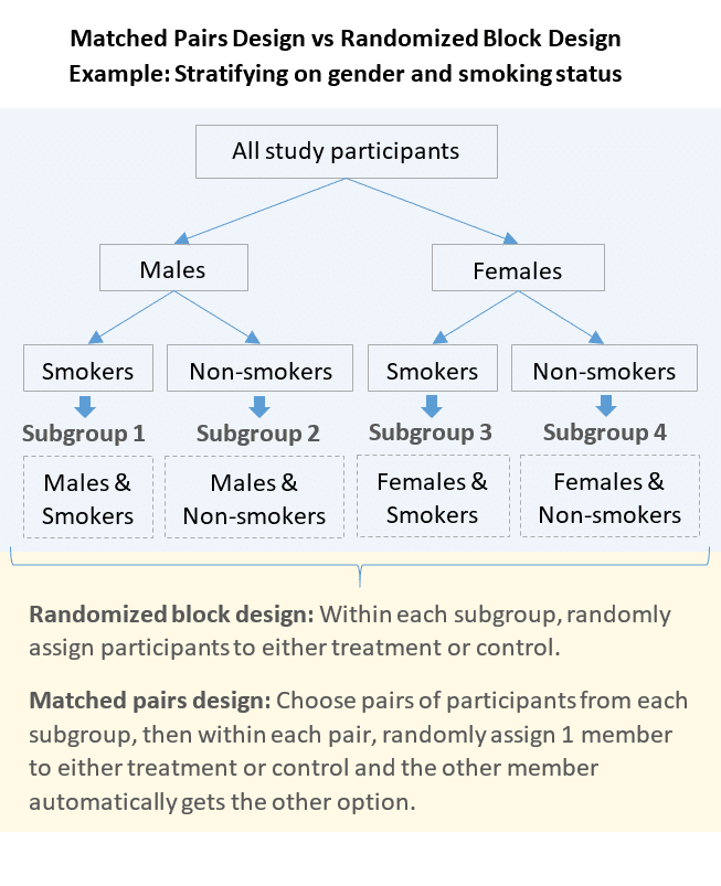
When working with a small sample, using simple randomization alone can produce, just by chance, unbalanced groups regarding the patients’ initial characteristics (for a detailed discussion see:   Purpose and Limitations of Random Assignment ). In these cases, ensuring equivalence between participants by using either a matched pairs design or a randomized block design will increase the statistical power and precision of the study.

Where randomized block design is better:

Matched pairs design may not be the best option in the following cases:

• If an eligible participant will have to wait a long time to be randomized because a suitable match is hard to find.
• If paired participants may not be similar regarding other important characteristics.
• If the subgroups have an odd number of participants. In this case, each will be left with 1 unpaired participant. Losing some participants this way can be problematic in cases where we are already working with a small sample, and/or very few participants are eligible for the study.

Where matched pairs design is better:

Matching is especially useful in cases where participants can be paired with themselves.

For instance, in order to study the effect of a new sunscreen, the new product can be applied to the right arm (the treatment group), and the left arm can be used as control.

Where a completely randomized design is better than both:

Neither matching nor blocking is necessary in studies with large sample sizes, since in these cases, simple randomization alone is enough to balance study groups.

• Friedman LM, Furberg CD, DeMets DL, Reboussin DM, Granger CB. Fundament als of Clinical Trials. 5th edition. Springer; 2015.
• Hulley SB, Cummings SR, Browner WS, Grady DG, Newman TB. Designing Clinical Research . 4th edition. LWW; 2013.

Further reading

• Randomized Block Design
• Matched Pairs Design
• Posttest-Only Control Group Design
• Pretest-Posttest Control Group Design

randomizr Easy-to-Use Tools for Common Forms of Random Assignment and Sampling

• Design and Analysis of Experiments with randomizr
• block_and_cluster_ra: Blocked and Clustered Random Assignment
• block_and_cluster_ra_probabilities: probabilities of assignment: Blocked and Clustered Random...
• block_ra: Block Random Assignment
• block_ra_probabilities: probabilities of assignment: Block Random Assignment
• cluster_ra: Cluster Random Assignment
• cluster_ra_probabilities: probabilities of assignment: Cluster Random Assignment
• cluster_rs: Cluster Random Sampling
• cluster_rs_probabilities: Inclusion Probabilities: Cluster Sampling
• complete_ra: Complete Random Assignment
• complete_ra_probabilities: probabilities of assignment: Complete Random Assignment
• complete_rs: Complete Random Sampling
• complete_rs_probabilities: Inclusion Probabilities: Complete Random Sampling
• conduct_ra: Conduct a random assignment
• custom_ra: Custom Random Assignment
• custom_ra_probabilities: probabilities of assignment: Custom Random Assignment
• declare_ra: Declare a random assignment procedure.
• declare_rs: Declare a random sampling procedure.
• draw_rs: Draw a random sample
• obtain_condition_probabilities: Obtain the probabilities of units being in the conditions...
• obtain_inclusion_probabilities: Obtain inclusion probabilities
• obtain_num_permutations: Obtain the Number of Possible Permutations from a Random...
• obtain_permutation_matrix: Obtain Permutation Matrix from a Random Assignment...
• obtain_permutation_probabilities: Obtain the probabilities of permutations
• randomizr: randomizr
• simple_ra: Simple Random Assignment
• simple_ra_probabilities: probabilities of assignment: Simple Random Assignment
• simple_rs: Simple Random Sampling
• simple_rs_probabilities: Inclusion Probabilities: Simple Random Sampling
• strata_and_cluster_rs: Stratified and Clustered Random Sampling
• strata_and_cluster_rs_probabilities: Inclusion Probabilities: Stratified and Clustered Random...
• strata_rs: Stratified Random Sampling
• strata_rs_probabilities: Inclusion Probabilities: Stratified Random Sampling
• Browse all...

block_ra : Block Random Assignment In randomizr: Easy-to-Use Tools for Common Forms of Random Assignment and Sampling

View source: R/block_ra.R

Block Random Assignment

Description.

block_ra implements a random assignment procedure in which units that are grouped into blocks defined by pre-treatment covariates are assigned using complete random assignment within block. For example, imagine that 50 of 100 men are assigned to treatment and 75 of 200 women are assigned to treatment.

A vector of length N that indicates the treatment condition of each unit. Is numeric in a two-arm trial and a factor variable (ordered by conditions) in a multi-arm trial.

Related to block_ra in randomizr ...

R package documentation, browse r packages, we want your feedback.

Add the following code to your website.

REMOVE THIS Copy to clipboard

For more information on customizing the embed code, read Embedding Snippets .

Blocked and Clustered Random Assignment

A random assignment procedure in which units are assigned as clusters and clusters are nested within blocks.

A vector of length N that indicates which block each unit belongs to.

A vector of length N that indicates which cluster each unit belongs to.

Use for a two-arm design in which either floor(N_clusters_block*prob) or ceiling(N_clusters_block*prob) clusters are assigned to treatment within each block. The probability of assignment to treatment is exactly prob because with probability 1-prob, floor(N_clusters_block*prob) clusters will be assigned to treatment and with probability prob, ceiling(N_clusters_block*prob) clusters will be assigned to treatment. prob must be a real number between 0 and 1 inclusive. (optional)

Use for a two arm design. Must of be of length N. tapply(prob_unit, blocks, unique) will be passed to block_prob .

Use for a multi-arm design in which the values of prob_each determine the probabilities of assignment to each treatment condition. prob_each must be a numeric vector giving the probability of assignment to each condition. All entries must be nonnegative real numbers between 0 and 1 inclusive and the total must sum to 1. Because of integer issues, the exact number of clusters assigned to each condition may differ (slightly) from assignment to assignment, but the overall probability of assignment is exactly prob_each. (optional)

Use for a two-arm design in which the scalar m describes the fixed number of clusters assigned in each block. This number does not vary across blocks.

Use for a two-arm design. Must be of length N. tapply(m_unit, blocks, unique) will be passed to block_m .

Use for a two-arm design in which block_m describes the number of clusters to assign to treatment within each block. block_m must be a numeric vector that is as long as the number of blocks and is in the same order as sort(unique(blocks)).

Use for a multi-arm design in which the values of block_m_each determine the number of clusters assigned to each condition. block_m_each must be a matrix with the same number of rows as blocks and the same number of columns as treatment arms. Cell entries are the number of clusters to be assigned to each treatment arm within each block. The rows should respect the ordering of the blocks as determined by sort(unique(blocks)). The columns should be in the order of conditions, if specified.

Use for a two-arm design in which block_prob describes the probability of assignment to treatment within each block. Must be in the same order as sort(unique(blocks)). Differs from prob in that the probability of assignment can vary across blocks.

Use for a multi-arm design in which the values of block_prob_each determine the probabilities of assignment to each treatment condition. block_prob_each must be a matrix with the same number of rows as blocks and the same number of columns as treatment arms. Cell entries are the probabilities of assignment to treatment within each block. The rows should respect the ordering of the blocks as determined by sort(unique(blocks)). Use only if the probabilities of assignment should vary by block, otherwise use prob_each. Each row of block_prob_each must sum to 1.

The number of treatment arms. If unspecified, num_arms will be determined from the other arguments. (optional)

A character vector giving the names of the treatment groups. If unspecified, the treatment groups will be named 0 (for control) and 1 (for treatment) in a two-arm trial and T1, T2, T3, in a multi-arm trial. An exception is a two-group design in which num_arms is set to 2, in which case the condition names are T1 and T2, as in a multi-arm trial with two arms. (optional)

logical. Defaults to TRUE.

A vector of length N that indicates the treatment condition of each unit.