7 1 spss assignment 3 scatterplots and correlations

• Flashes Safe Seven
• FlashLine Login
• Faculty & Staff Phone Directory
• Emeriti or Retiree
• All Departments
• Maps & Directions

• Building Guide
• Departments
• Directions & Parking
• Faculty & Staff
• Give to University Libraries
• Library Instructional Spaces
• Mission & Vision
• Newsletters
• Circulation
• Course Reserves / Core Textbooks
• Equipment for Checkout
• Interlibrary Loan
• Library Instruction
• Library Tutorials
• My Library Account
• Open Access Kent State
• Research Support Services
• Statistical Consulting
• Student Multimedia Studio
• Citation Tools
• Databases A-to-Z
• Databases By Subject
• Digital Collections
• Discovery@Kent State
• Government Information
• Journal Finder
• Library Guides
• Connect from Off-Campus
• Library Workshops
• Subject Librarians Directory
• Suggestions/Feedback
• Writing Commons
• Academic Integrity
• Jobs for Students
• International Students
• Meet with a Librarian
• Study Spaces
• University Libraries Student Scholarship
• Affordable Course Materials
• Copyright Services
• Selection Manager
• Suggest a Purchase

Library Locations at the Kent Campus

• Architecture Library
• Fashion Library
• Map Library
• Performing Arts Library
• Special Collections and Archives

Regional Campus Libraries

• East Liverpool
• College of Podiatric Medicine

• Kent State University
• SPSS Tutorials

Pearson Correlation

Spss tutorials: pearson correlation.

• The SPSS Environment
• The Data View Window
• Using SPSS Syntax
• Data Creation in SPSS
• Importing Data into SPSS
• Variable Types
• Date-Time Variables in SPSS
• Defining Variables
• Creating a Codebook
• Computing Variables
• Computing Variables: Mean Centering
• Computing Variables: Recoding Categorical Variables
• Computing Variables: Recoding String Variables into Coded Categories (Automatic Recode)
• rank transform converts a set of data values by ordering them from smallest to largest, and then assigning a rank to each value. In SPSS, the Rank Cases procedure can be used to compute the rank transform of a variable." href="https://libguides.library.kent.edu/SPSS/RankCases" style="" >Computing Variables: Rank Transforms (Rank Cases)
• Weighting Cases
• Sorting Data
• Grouping Data
• Descriptive Stats for One Numeric Variable (Explore)
• Descriptive Stats for One Numeric Variable (Frequencies)
• Descriptive Stats for Many Numeric Variables (Descriptives)
• Descriptive Stats by Group (Compare Means)
• Frequency Tables
• Working with "Check All That Apply" Survey Data (Multiple Response Sets)
• Chi-Square Test of Independence
• One Sample t Test
• Paired Samples t Test
• Independent Samples t Test
• One-Way ANOVA
• How to Cite the Tutorials

Sample Data Files

Our tutorials reference a dataset called "sample" in many examples. If you'd like to download the sample dataset to work through the examples, choose one of the files below:

• Data definitions (*.pdf)
• Data - Comma delimited (*.csv)
• Data - Tab delimited (*.txt)
• Data - Excel format (*.xlsx)
• Data - SAS format (*.sas7bdat)
• Data - SPSS format (*.sav)
• SPSS Syntax (*.sps) Syntax to add variable labels, value labels, set variable types, and compute several recoded variables used in later tutorials.
• SAS Syntax (*.sas) Syntax to read the CSV-format sample data and set variable labels and formats/value labels.

The bivariate Pearson Correlation produces a sample correlation coefficient, r , which measures the strength and direction of linear relationships between pairs of continuous variables. By extension, the Pearson Correlation evaluates whether there is statistical evidence for a linear relationship among the same pairs of variables in the population, represented by a population correlation coefficient, ρ (“rho”). The Pearson Correlation is a parametric measure.

This measure is also known as:

• Pearson’s correlation
• Pearson product-moment correlation (PPMC)

Common Uses

The bivariate Pearson Correlation is commonly used to measure the following:

• Correlations among pairs of variables
• Correlations within and between sets of variables

The bivariate Pearson correlation indicates the following:

• Whether a statistically significant linear relationship exists between two continuous variables
• The strength of a linear relationship (i.e., how close the relationship is to being a perfectly straight line)
• The direction of a linear relationship (increasing or decreasing)

Note: The bivariate Pearson Correlation cannot address non-linear relationships or relationships among categorical variables. If you wish to understand relationships that involve categorical variables and/or non-linear relationships, you will need to choose another measure of association.

Note: The bivariate Pearson Correlation only reveals associations among continuous variables. The bivariate Pearson Correlation does not provide any inferences about causation, no matter how large the correlation coefficient is.

Data Requirements

To use Pearson correlation, your data must meet the following requirements:

• Two or more continuous variables (i.e., interval or ratio level)
• Cases must have non-missing values on both variables
• Linear relationship between the variables
• the values for all variables across cases are unrelated
• for any case, the value for any variable cannot influence the value of any variable for other cases
• no case can influence another case on any variable
• The biviariate Pearson correlation coefficient and corresponding significance test are not robust when independence is violated.
• Each pair of variables is bivariately normally distributed
• Each pair of variables is bivariately normally distributed at all levels of the other variable(s)
• This assumption ensures that the variables are linearly related; violations of this assumption may indicate that non-linear relationships among variables exist. Linearity can be assessed visually using a scatterplot of the data.
• Random sample of data from the population
• No outliers

The null hypothesis ( H 0 ) and alternative hypothesis ( H 1 ) of the significance test for correlation can be expressed in the following ways, depending on whether a one-tailed or two-tailed test is requested:

Two-tailed significance test:

H 0 : ρ  = 0 ("the population correlation coefficient is 0; there is no association") H 1 : ρ ≠ 0 ("the population correlation coefficient is not 0; a nonzero correlation could exist")

One-tailed significance test:

H 0 : ρ  = 0 ("the population correlation coefficient is 0; there is no association") H 1 : ρ   > 0 ("the population correlation coefficient is greater than 0; a positive correlation could exist")      OR H 1 : ρ   < 0 ("the population correlation coefficient is less than 0; a negative correlation could exist")

where ρ is the population correlation coefficient.

Test Statistic

The sample correlation coefficient between two variables x and y is denoted r or r xy , and can be computed as: $$ r_{xy} = \frac{\mathrm{cov}(x,y)}{\sqrt{\mathrm{var}(x)} \dot{} \sqrt{\mathrm{var}(y)}} $$

where cov( x , y ) is the sample covariance of x and y ; var( x ) is the sample variance of x ; and var( y ) is the sample variance of y .

Correlation can take on any value in the range [-1, 1]. The sign of the correlation coefficient indicates the direction of the relationship, while the magnitude of the correlation (how close it is to -1 or +1) indicates the strength of the relationship.

•  -1 : perfectly negative linear relationship
•   0 : no relationship
• +1  : perfectly positive linear relationship

The strength can be assessed by these general guidelines [1] (which may vary by discipline):

• .1 < | r | < .3 … small / weak correlation
• .3 < | r | < .5 … medium / moderate correlation
• .5 < | r | ……… large / strong correlation

Note: The direction and strength of a correlation are two distinct properties. The scatterplots below [2] show correlations that are r = +0.90, r = 0.00, and r = -0.90, respectively. The strength of the nonzero correlations are the same: 0.90. But the direction of the correlations is different: a negative correlation corresponds to a decreasing relationship, while and a positive correlation corresponds to an increasing relationship. 

Note that the r = 0.00 correlation has no discernable increasing or decreasing linear pattern in this particular graph. However, keep in mind that Pearson correlation is only capable of detecting linear associations, so it is possible to have a pair of variables with a strong nonlinear relationship and a small Pearson correlation coefficient. It is good practice to create scatterplots of your variables to corroborate your correlation coefficients.

[1]  Cohen, J. (1988). Statistical power analysis for the behavioral sciences (2nd ed.). Hillsdale, NJ: Lawrence Erlbaum Associates.

[2]  Scatterplots created in R using ggplot2 , ggthemes::theme_tufte() , and MASS::mvrnorm() .

Data Set-Up

Your dataset should include two or more continuous numeric variables, each defined as scale, which will be used in the analysis.

Each row in the dataset should represent one unique subject, person, or unit. All of the measurements taken on that person or unit should appear in that row. If measurements for one subject appear on multiple rows -- for example, if you have measurements from different time points on separate rows -- you should reshape your data to "wide" format before you compute the correlations.

Run a Bivariate Pearson Correlation

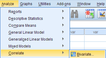
To run a bivariate Pearson Correlation in SPSS, click  Analyze > Correlate > Bivariate .

The Bivariate Correlations window opens, where you will specify the variables to be used in the analysis. All of the variables in your dataset appear in the list on the left side. To select variables for the analysis, select the variables in the list on the left and click the blue arrow button to move them to the right, in the Variables field.

A Variables : The variables to be used in the bivariate Pearson Correlation. You must select at least two continuous variables, but may select more than two. The test will produce correlation coefficients for each pair of variables in this list.

B Correlation Coefficients: There are multiple types of correlation coefficients. By default, Pearson is selected. Selecting Pearson will produce the test statistics for a bivariate Pearson Correlation.

C Test of Significance:  Click Two-tailed or One-tailed , depending on your desired significance test. SPSS uses a two-tailed test by default.

D Flag significant correlations: Checking this option will include asterisks (**) next to statistically significant correlations in the output. By default, SPSS marks statistical significance at the alpha = 0.05 and alpha = 0.01 levels, but not at the alpha = 0.001 level (which is treated as alpha = 0.01)

E Options : Clicking Options will open a window where you can specify which Statistics to include (i.e., Means and standard deviations , Cross-product deviations and covariances ) and how to address Missing Values (i.e., Exclude cases pairwise or Exclude cases listwise ). Note that the pairwise/listwise setting does not affect your computations if you are only entering two variable, but can make a very large difference if you are entering three or more variables into the correlation procedure.

Example: Understanding the linear association between weight and height

Problem statement.

Perhaps you would like to test whether there is a statistically significant linear relationship between two continuous variables, weight and height (and by extension, infer whether the association is significant in the population). You can use a bivariate Pearson Correlation to test whether there is a statistically significant linear relationship between height and weight, and to determine the strength and direction of the association.

Before the Test

In the sample data, we will use two variables: “Height” and “Weight.” The variable “Height” is a continuous measure of height in inches and exhibits a range of values from 55.00 to 84.41 ( Analyze > Descriptive Statistics > Descriptives ). The variable “Weight” is a continuous measure of weight in pounds and exhibits a range of values from 101.71 to 350.07.

Before we look at the Pearson correlations, we should look at the scatterplots of our variables to get an idea of what to expect. In particular, we need to determine if it's reasonable to assume that our variables have linear relationships. Click Graphs > Legacy Dialogs > Scatter/Dot . In the Scatter/Dot window, click Simple Scatter , then click Define . Move variable Height to the X Axis box, and move variable Weight to the Y Axis box. When finished, click OK .

To add a linear fit like the one depicted, double-click on the plot in the Output Viewer to open the Chart Editor. Click Elements > Fit Line at Total . In the Properties window, make sure the Fit Method is set to Linear , then click Apply . (Notice that adding the linear regression trend line will also add the R-squared value in the margin of the plot. If we take the square root of this number, it should match the value of the Pearson correlation we obtain.)

From the scatterplot, we can see that as height increases, weight also tends to increase. There does appear to be some linear relationship.

Running the Test

To run the bivariate Pearson Correlation, click  Analyze > Correlate > Bivariate . Select the variables Height and Weight and move them to the Variables box. In the Correlation Coefficients area, select Pearson . In the Test of Significance area, select your desired significance test, two-tailed or one-tailed. We will select a two-tailed significance test in this example. Check the box next to Flag significant correlations .

Click OK to run the bivariate Pearson Correlation. Output for the analysis will display in the Output Viewer.

The results will display the correlations in a table, labeled Correlations .

A Correlation of Height with itself (r=1), and the number of nonmissing observations for height (n=408).

B Correlation of height and weight (r=0.513), based on n=354 observations with pairwise nonmissing values.

C Correlation of height and weight (r=0.513), based on n=354 observations with pairwise nonmissing values.

D Correlation of weight with itself (r=1), and the number of nonmissing observations for weight (n=376).

The important cells we want to look at are either B or C. (Cells B and C are identical, because they include information about the same pair of variables.) Cells B and C contain the correlation coefficient for the correlation between height and weight, its p-value, and the number of complete pairwise observations that the calculation was based on.

The correlations in the main diagonal (cells A and D) are all equal to 1. This is because a variable is always perfectly correlated with itself. Notice, however, that the sample sizes are different in cell A ( n =408) versus cell D ( n =376). This is because of missing data -- there are more missing observations for variable Weight than there are for variable Height.

If you have opted to flag significant correlations, SPSS will mark a 0.05 significance level with one asterisk (*) and a 0.01 significance level with two asterisks (0.01). In cell B (repeated in cell C), we can see that the Pearson correlation coefficient for height and weight is .513, which is significant ( p < .001 for a two-tailed test), based on 354 complete observations (i.e., cases with nonmissing values for both height and weight).

Decision and Conclusions

Based on the results, we can state the following:

• Weight and height have a statistically significant linear relationship ( r =.513, p < .001).
• The direction of the relationship is positive (i.e., height and weight are positively correlated), meaning that these variables tend to increase together (i.e., greater height is associated with greater weight).
• The magnitude, or strength, of the association is approximately moderate (.3 < | r | < .5).
• << Previous: Chi-Square Test of Independence
• Next: One Sample t Test >>
• Last Updated: Jun 14, 2024 11:54 AM
• URL: https://libguides.library.kent.edu/SPSS

Street Address

Mailing address, quick links.

• How Are We Doing?
• Student Jobs

Information

• Accessibility
• Emergency Information
• For Our Alumni
• For the Media
• Jobs & Employment
• Life at KSU
• Privacy Statement
• Technology Support
• Website Feedback

Pardon Our Interruption

As you were browsing something about your browser made us think you were a bot. There are a few reasons this might happen:

• You've disabled JavaScript in your web browser.
• You're a power user moving through this website with super-human speed.
• You've disabled cookies in your web browser.
• A third-party browser plugin, such as Ghostery or NoScript, is preventing JavaScript from running. Additional information is available in this support article .

To regain access, please make sure that cookies and JavaScript are enabled before reloading the page.

If you're seeing this message, it means we're having trouble loading external resources on our website.

If you're behind a web filter, please make sure that the domains *.kastatic.org and *.kasandbox.org are unblocked.

To log in and use all the features of Khan Academy, please enable JavaScript in your browser.

Statistics and probability

Course: statistics and probability   >   unit 5.

• Constructing a scatter plot
• Constructing scatter plots
• Making appropriate scatter plots
• Example of direction in scatterplots
• Scatter plot: smokers
• Bivariate relationship linearity, strength and direction
• Positive and negative linear associations from scatter plots
• Describing trends in scatterplots
• Positive and negative associations in scatterplots
• Outliers in scatter plots
• Clusters in scatter plots
• Describing scatterplots (form, direction, strength, outliers)

Scatterplots and correlation review

What is a scatterplot?

What is correlation.

• (Choice A)   Positive linear correlation A Positive linear correlation
• (Choice B)   Negative linear correlation B Negative linear correlation
• (Choice C)   No association C No association

Want to join the conversation?

• Upvote Button navigates to signup page
• Downvote Button navigates to signup page
• Flag Button navigates to signup page

Answering questions with data: Lab Manual

Chapter 3 Lab 3: Correlation

If … we choose a group of social phenomena with no antecedent knowledge of the causation or absence of causation among them, then the calculation of correlation coefficients, total or partial, will not advance us a step toward evaluating the importance of the causes at work. —Sir Ronald Fisher

In lecture and in the textbook, we have been discussing the idea of correlation. This is the idea that two things that we measure can be somehow related to one another. For example, your personal happiness, which we could try to measure say with a questionnaire, might be related to other things in your life that we could also measure, such as number of close friends, yearly salary, how much chocolate you have in your bedroom, or how many times you have said the word Nintendo in your life. Some of the relationships that we can measure are meaningful, and might reflect a causal relationship where one thing causes a change in another thing. Some of the relationships are spurious, and do not reflect a causal relationship.

In this lab you will learn how to compute correlations between two variables in software, and then ask some questions about the correlations that you observe.

3.1 General Goals

• Compute Pearson’s r between two variables using software
• Discuss the possible meaning of correlations that you observe

3.1.1 Important Info

We use data from the World Happiness Report . A .csv of the data can be found here: WHR2018.csv

In this lab we use explore to explore correlations between any two variables, and also show how to do a regression line. There will be three main parts. Getting R to compute the correlation, and looking at the data using scatter plots. We’ll look at some correlations from the World Happiness Report. Then you’ll look at correlations using data we collect from ourselves. It will be fun.

3.2.1 cor for correlation

R has the cor function for computing Pearson’s r between any two variables. In fact this same function computes other versions of correlation, but we’ll skip those here. To use the function you just need two variables with numbers in them like this:

Well, that was easy.

3.2.1.1 scatterplots

Let’s take our silly example, and plot the data in a scatter plot using ggplot2, and let’s also return the correlation and print it on the scatter plot. Remember, ggplot2 wants the data in a data.frame, so we first put our x and y variables in a data frame.

Wow, we’re moving fast here.

3.2.1.2 lots of scatterplots

Before we move on to real data, let’s look at some fake data first. Often we will have many measures of X and Y, split between a few different conditions, for example, A, B, C, and D. Let’s make some fake data for X and Y, for each condition A, B, C, and D, and then use facet_wrapping to look at four scatter plots all at once

3.2.1.3 computing the correlations all at once

We’ve seen how we can make four graphs at once. Facet_wrap will always try to make as many graphs as there are individual conditions in the column variable. In this case there are four, so it makes four.

Notice, the scatter plots don’t show the correlation (r) values. Getting these numbers on there is possible, but we have to calculate them first. We’ll leave it to you to Google how to do this, if it’s something you want to do. Instead, what we will do is make a table of the correlations in addition to the scatter plot. We again use dplyr to do this:

OK, we are basically ready to turn to some real data and ask if there are correlations between interesting variables…You will find that there are some… But before we do that, we do one more thing. This will help you become a little bit more skeptical of these “correlations”.

3.2.1.4 Chance correlations

As you learned from the textbook. We can find correlations by chance alone, even when there is no true correlation between the variables. For example, if we sampled randomly into x, and then sampled some numbers randomly into y. We know they aren’t related, because we randomly sampled the numbers. However, doing this creates some correlations some of the time just by chance. You can demonstrate this to yourself with the following code. It’s a repeat of what we already saw, jut with a few more conditions added. Let’s look at 20 conditions, with random numbers for x and y in each. For each, sample size will be 10. We’ll make the fake data, then make a big graph to look at all. And, even though we get to regression later in the lab, I’ll put the best fit line onto each scatter plot, so you can “see the correlations”.

You can see that the slope of the blue line is not always flat. Sometimes it looks like there is a correlation, when we know there shouldn’t be. You can keep re-doing this graph, by re-knitting your R Markdown document, or by pressing the little green play button. This is basically you simulating the outcomes as many times as you press the button.

The point is, now you know you can find correlations by chance. So, in the next section, you should always wonder if the correlations you find reflect meaningful association between the x and y variable, or could have just occurred by chance.

3.2.2 World Happiness Report

Let’s take a look at some correlations in real data. We are going to look at responses to a questionnaire about happiness that was sent around the world, from the world happiness report

3.2.2.1 Load the data

We load the data into a data frame. Reminder, the following assumes that you have downloaded the RMarkdownsLab.zip file which contains the data file in the data folder.

You can also load the data using the following URL

3.2.2.2 Look at the data

You should be able to see that there is data for many different countries, across a few different years. There are lots of different kinds of measures, and each are given a name. I’ll show you some examples of asking questions about correlations with this data, then you get to ask and answer your own questions.

3.2.2.3 My Question #1

For the year 2017 only, does a countries measure for “freedom to make life choices” correlate with that countries measure for " Confidence in national government"?

Let’s find out. We calculate the correlation, and then we make the scatter plot.

Interesting, what happened here? We can see some dots, but the correlation was NA (meaning undefined). This occurred because there are some missing data points in the data. We can remove all the rows with missing data first, then do the correlation. We will do this a couple steps, first creating our own data.frame with only the numbers we want to analyse. We can select the columns we want to keep using select . Then we use filter to remove the rows with NAs.

Now we see the correlation is .408.

Although the scatter plot shows the dots are everywhere, it generally shows that as Freedom to make life choices increases in a country, that countries confidence in their national government also increase. This is a positive correlation. Let’s do this again and add the best fit line, so the trend is more clear, we use geom_smooth(method=lm, se=FALSE) . I also change the alpha value of the dots so they blend it bit, and you can see more of them.

3.2.2.4 My Question #2

After all that work, we can now speedily answer more questions. For example, what is the relationship between positive affect in a country and negative affect in a country. I wouldn’t be surprised if there was a negative correlation here: when positive feelings generally go up, shouldn’t negative feelings generally go down?

To answer this question, we just copy paste the last code block, and change the DVs to be Positive affect , and Negative affect

Bam, there we have it. As positive affect goes up, negative affect goes down. A negative correlation.

3.2.3 Generalization Exercise

This generalization exercise will explore the idea that correlations between two measures can arise by chance alone. There are two questions to answer. For each question you will be sampling random numbers from uniform distribution. To conduct the estimate, you will be running a simulation 100 times. The questions are:

Estimate the range (minimum and maximum) of correlations (using pearons’s r) that could occur by chance between two variables with n=10.

Estimate the range (minimum and maximum) of correlations (using pearons’s r) that could occur bychance between two variables with n = 100.

Use these tips to answer the question.

Tip 1: You can use the runif() function to sample random numbers between a minimum value, and maximum value. The example below sample 10 (n=10) random numbers between the range 0 (min = 0) and 10 (max=10). Everytime you run this code, the 10 values in x will be re-sampled, and will be 10 new random numbers

Tip 2: You can compute the correlation between two sets of random numbers, by first sampling random numbers into each variable, and then running the cor() function.

Running the above code will give different values for the correlation each time, because the numbers in x and y are always randomly different. We might expect that because x and y are chosen randomly that there should be a 0 correlation. However, what we see is that random sampling can produce “fake” correlations just by chance alone. We want to estimate the range of correlations that chance can produce.

Tip 3: One way to estimate the range of correlations that chance can produce is to repeat the above code many times. For example, if you ran the above code 100 times, you could save the correlations each time, then look at the smallest and largest correlation. This would be an estimate of the range of correlations that can be produced by chance. How can you repeat the above code many times to solve this problem?

We can do this using a for loop. The code below shows how to repeat everything inside the for loop 100 times. The variable i is an index, that goes from 1 to 100. The saved_value variable starts out as an empty variable, and then we put a value into it (at index position i, from 1 to 100). In this code, we put the sum of the products of x and y into the saved_value variable. At the end of the simulation, the save_value variable contains 100 numbers. The min() and max() functions are used to find the minimum and maximum values for each of the 100 simulations. You should be able to modify this code by replacing sum(x*y) with cor(x,y) . Doing this will allow you to run the simulation 100 times, and find the minimum correlation and maximum correlation that arises by chance. This will be estimate for question 1. To provide an estimate for question 2, you will need to change n=10 to n=100 .

3.2.4 Writing assignment

Answer the following questions with complete sentences. When you have finished everything. Knit the document and hand in your stuff (you can submit your .RMD file to blackboard if it does not knit.)

Imagine a researcher found a positive correlation between two variables, and reported that the r value was +.3. One possibility is that there is a true correlation between these two variables. Discuss one alternative possibility that would also explain the observation of +.3 value between the variables.

Explain the difference between a correlation of r = .3 and r = .7. What does a larger value of r represent?

Explain the difference between a correlation of r = .5, and r = -.5.

How to do it in Excel

In this lab, we will use SPSS to calculate the correlation coefficient. We will focus on the most-commonly used Pearson’s coefficient, r. We will learn how to:

• Calculate the Pearson’s r correlation coefficient for bivariate data
• Produce a correlation matrix, reporting Pearson’s r for more than two variables at a time
• Produce a scatterplot
• Split a data file for further analysis

Let’s first begin with a short data set we will enter into a new SPSS data spreadsheet. Remember, in order to calculate a correlation, you need to have bivariate data; that is, you must have at least two variables, x and y. You can have more than two variables, in which case we can calculate a correlation matrix, as indicated in the section that follows.

3.4.1 Correlation Coefficient for Bivariate Data: Two Variables

Let’s use the following data set: {x= 1, 3, 2, 5, 4, 6, 5, 8, 9} {y= 6, 5, 8, 7, 9, 7, 8, 10, 13}. Notice there are two variables, x and y . Enter these into SPSS and name them appropriately.

Next, click Analyze , then Correlate , then Bivariate :

The next window will ask you to select variables to correlate. Since we have two ( x and y ) move them both from the left-hand field to the right-hand field using the arrow. Notice that in this window, Pearson is selected. This is the default setting (and the one we want), but notice there are other ways to calculate the correlation between variables. We will stick with Pearson’s correlation coefficient for this course.

Now, click OK .

SPSS will produce an output table containing the correlation coefficient requested. Notice that the table is redundant; it gives us the correlation between x and y, the correlation between y and x, the correlation between x and itself, and the correlation between y and itself. Any variable correlated with itself will result in an r of 1. The Pearson r correlation between variables x and y is .765.

3.4.2 Correlation Matrix

In the event that you have more than two variables in your spreadsheet, and would like to evaluate correlations between several variables taken two at a time, you need not re-run the correlations in SPSS repeatedly. You can, in fact, enter multiple variables into the correlation window and obtain a correlation matrix–a table showing every possible bivariate correlation amongst a group of variables.

From here, go to Analyze , then Correlate , then Bivariate :

Next, you will encounter the window that asks you to indicate which variables to correlate. Select all three variables ( x , y , and z ) and move them to the right-hand field using the arrow.

Click OK . SPSS will produce an output table that contains correlations for every pairing of our three variables, along with the correlations of each variable with itself.

According to this output:

• The correlation coefficient between variables x and y is .765
• The correlation coefficient between variables x and z is .294
• The correlation coefficient between variables y and z is -.080

3.4.3 Correlation and Scatterplots

To accompany the calculation of the correlation coefficient, the scatterplot is the relevant visualization tool. Let’s use data from The World Happiness Report, a questionnaire about happiness. Here is a link to the file named WHR2018.sav.

Using this data, let’s answer the following question: does a country’s measure for freedom to make life choices correlate with that country’s measure for Confidence in national government ?

Let’s find the correlation coefficient between these variables first. Go to Analyze , then Correlate , then Bivariate :

Next, a window will appear asking for the variables to be correlated. Go through the list on the left and find Freedom to make life choices as well as Confidence in national government . Move both of these variables to the field on the right using the arrow.

Based on this output, the correlation between Freedom to make life choices and Confidence in national government is .408.

Next, move your two variables ( freedom to make life choices and confidence in national government ) into the x-axis and y-axis fields. Again, it does not matter which variable goes where, for now.

Click OK . SPSS will produce a scatterplot of your data, as follows:

You can keep this scatterplot as it is, or, you can edit it to include a straight line that best fits the data points. This line is known as the best-fitting line as it minimizes the distance from it to all the data. To edit the scatterplot double click on the graph and a window labeled Chart Editor should appear:

In this window, find the button at the top that reads Fit Line at Total when you hover your mouse over it. Below, I have highlighted it for clarity:

Press this button and you will see a new menu. Make sure Linear is selected and click Apply .

Next, exit from the Chart Editor. This means you will hit the X in the corner of the window. You will find that the graph in your output window has now updated and has a line drawn on it.

This scatterplot is very important. The distance between the line and the data points is indicative of the strength of the correlation coefficient; they are directly related. For example, if the data were more clustered or tighter to the line, the correlation would be stronger. If the data points are more spread out and far from the line, the correlation is weaker.

3.4.4 Splitting a File

What if we asked the question: for the year 2017 only, does a countries measure for freedom to make life choices correlate with that countries measure for Confidence in national government ?

Notice that this question is asking us to find the correlation between the same two variables we used in the previous example, but only in the case where the year is 2017. To acheive this, we’re going to utilize a function called splitting. Splitting takes the file as a whole, and sets it up so that every analysis is done on some subset of the data. For example, if we split our data by year and calculate a correlation coefficient, SPSS will find Pearson r for only 2017, and another for only 2016, and so on.

In order to split the data, we go to the top menu and choose Data , then Split file…

In the next window, you must select Organize output by groups and then specify which variable will be used to split the data. Select year and move it to the right-hand field using the arrow.

Click OK . Notice that this will cause the output window to produce some next indicating that you have split your file. You can ignore this and go back to your data window.

From here, any analysis you choose to do will be done separately for each year’s worth of data. Let’s calculate the correlation coefficient, as usual. Click Analyze , then Correlate , then Bivariate :

In the next window, select the variables to be used (they will be the same as in the last example).

Click OK . Notice that in the output window you will see a bunch of correlation tables (13 of them to be exact); one for each year. Scroll down and find the table with the heading “year = 2017”. That’s the table we need in order to answer our question:

This table indicates that, if we only look at the year 2017, the correlation coefficient between freedom to make life choices and confidence in national government is .442.

It is VERY important to remember that once you have split a file, every analysis that follows the split will be done on the split variable. If you want to go back to performing analyses and calculating statistics for the data as a whole, you must UNSPLIT your data file (or undo the split). To do this, go to Data , then Split file…

Then make sure to select Analyze all cases, do not create groups and click OK .

3.4.5 Practice Problems

For the year 2005 ONLY, find the correlation between “perceptions of corruption” and “positive affect”. Create a scatterplot to visualize this relationship. What are your conclusions about the relationship between affect and perceived corruption? Is this surprising to you?

What has happened to log GDP (consider this a measure of GDP) in the United States ONLY with time (as the year has increased)? Explain this relationship and provide a scatterplot.

Which country (or countries) have seen a more consistent and strong increase in log GDP over time? Which country (or countries) have seen a decrease over time?

How to do it in JAMOVI

Snapsolve any problem by taking a picture. Try it in the Numerade app?