2d representation of 3d objects

• Visualisation of 3D Objects in 2D

You must have seen the objects you are of different shapes and sizes. You are always surrounded by shapes like triangles, squares and circles. Have you ever observed the shape of your house? They have length, breadth and height and so they are called as 3 dimensional or 3D shapes. Let us now learn more about them. Let’s do it right now.

Suggested Videos

What are 2d objects.

2 -D figures are nothing but the two-dimensional figures. A shape or a figure that has a length and a breadth only is a 2D shape. The sides are made of straight or curved lines. They can have any number of sides. Triangle and squares are the examples of 2D objects. We will classify figures we have seen in terms of what is known as the dimension.

A plane object that has a length and a breadth only have 2 Dimensions. They can be drawn on a screen or a paper. The following are the examples of 2D objects.

3-D figures are nothing but the three-dimensional figures. In our day to day life, we see several objects like books, ball, ice-cream cone etc, around us which have different shapes. One thing common to most of these objects is that they all have some length, breadth and height or depth.

Therefore they all occupy space and have three dimensions. These objects cannot be drawn onscreen as it is a three-dimensional figure. The following are the examples of 3D objects.

Nets for Building 3D Shapes

“A net is a two-dimensional representation of a three-dimensional figure that is unfolded along its edges so that each face the figure is shown in two dimensions. In other words, a net is a pattern made when the surface of a three-dimensional figure is laid out felt showing each face of the figure.”  You have different nets for the different shape.

Different Views of 3D Shapes

There are different views of 3D shapes such as top view and side view.

For example, the top view of a cylinder will be a circle but its side view will be a rectangle.

Isometric Sketch

Isometric sketch of any shape is a 3D projection of that shape and all its lines are parallel to the major axis. Also, the lines are measurable. For example,

Three cubes each with 3 cm edge placed side by side to form a cuboid. Sketch an isometric sketch of this cuboid and find dimensions of the cuboid in cm.

Solution: Three cubes are side by side to form a cuboid. So, only one of the dimension change and the other two will remain the same. Two out of three dimensions of the cuboid will be 2 and the third will be 2 + 2 + 2 = 6. Thus, the dimensions of the cuboid are 2 × 2× 6

Solved Examples for You

Question 2: What cross-sections do you get when you cut a candle horizontally?

Answer : C is the correct option. You get a circle when you cut a candle horizontally.

Question 2: A bulb is burning just right above the ball. Name the shape of the shadow obtained.

Answer : A is the correct option. The shape of the shadow obtained will be of a ball.

Question 3: What are 3d shapes examples?

Answer: A cube, sphere, cone, rectangular prism, and cylinder are the basic 3-dimensional shapes that we observe around us. One can observe a cube in a Rubik’s cube as well as a die. Similarly, one can observe a rectangular prism in a box and a book. Also, a sphere can be observed in a globe while cone can be observed in a cone in a carrot.

Question 4: Explain the definition of 3d shapes?

Answer: 3D shapes refer to solid objects that consist of three dimensions. These dimensions are length, height, and width. 3D shapes objects happen to have depth to them.

Question 5: Explain what is a 3d triangle?

Answer: The tetrahedron refers to the three-dimensional case of the general concept of a Euclidean simplex. Furthermore, one may thus also call it as a 3-simplex. In the case of a tetrahedron, the base happens to be a triangle.  Therefore, a tetrahedron is also called as a “triangular pyramid”.

Question 6: Explain the face on a 3d shape?

Customize your course in 30 seconds

Which class are you in.

Boxes and Sketches

Leave a reply cancel reply.

Your email address will not be published. Required fields are marked *

Download the App

All About Maths

2d representations of 3d shapes; drawing and constructing shapes; loci (higher - unit 3).

• Teaching guidance

Teaching resources

• Exam resources

Specification references (in recommended teaching order)

Lesson plans, supplementary resources, homework sheets.

Please note that, due to the overlap of C/D questions, some material may have been tagged as appropriate for both Foundation and Higher tier. Equally, due to the nature of some questions, different parts of a question may assess different topics. Teachers are advised to ensure learners have covered all of the question content before using such questions.

Create, edit, and share assessments quickly and easily with Exampro Mathematics

Quick links

• AQA exams and results services

Registration Required

Tech Differences

Know the Technical Differences

Difference Between 2D and 3D Shapes

These are very common terms and frequently heard overtimes. We use 2 and 3 dimensions in several areas such as in engineering drawing, computer graphics, animations, and in real life too. In this article, we are going to understand the difference between 2D and 3D shapes.

Content: 2D Shapes Vs 3D Shapes

Comparison chart.

• Key Differences

Definition of 2D Shapes

We can consider that the shapes which can be produced on a flat surface are said to be 2D (dimensional) Shape. In other words, the shapes that only have length and width are the 2D shapes.

Now, what a 2D shape is? Before understanding the 2D shape, we must know what a 0D object is, which means there is no dimensions. A 0D shape is defined by a point.

Applications

All the parallel projections and one-point perspective projections in plans of some object are made in 2D. Geological maps also made in 2 dimensions, in which we use the method of contouring to show the depth with the help of different shapes, even in oceanography also.

Definition of 3D Shapes

3D shapes are solid shapes, unlike 2D shapes which are produced by combining 3 Dimensions – length, width and height. The real-life examples of these shapes are buildings, balls, boxes, anything that has 3 dimensions. Let’s consider a cuboidal building which is built with length, width and height is a 3D shape.

These are used in several applications, such as in 3D animations, 3D designing of some product building, bridge, tools, 3D graphs, maps etcetera. The 3D shapes help in showing the depth of the object. To illustrate the 3D in engineering, we use 2 and 3 point perspective projection and orthographic projection.

Key Differences Between 2D and 3D Shapes

• The prior difference between the 2D and 3D shapes is that in 2D shapes only two axis are incorporated x and y-axis. On the other hand, in 3D shapes, the three axis x, y and z-axis are covered.
• Square, circle, triangle, rectangle are the various 2D shapes while cube, sphere, cuboid, are the 3D shapes.
• The plan in engineering drawing, which represents in top view, front view side view of some object are made in 2D. Hence we use 2D shapes in these type of plans. Conversely, for representing three dimensions, the isometric and orthographic projections are used for rendering the 3D objects.
• We can use the manual or automatic methods of creating the 2D and 3D shapes, and there are several softwares used for doing this. However, 2D shapes are easy to create, whereas 3D shapes are challenging to build.
• The 2D shapes show all the edges of that shape, but in 3D shapes, these edges could be hidden. For example, in a square, all the edges are visible. However, if we take an example of the cube, then, it is not possible to display all of its edges from one angle.

From the above discussion, the basic difference between 2D and 3D shapes must be clear to you. So, 2D shapes are elementary flat shapes and have only 2 dimensions – x and y-axis. In contrast, 3D shapes contain three dimensions – x, y and z, in other terms these shapes have the volume too.

Related Differences:

• Difference Between View and Materialized View
• Difference Between Forward Engineering and Reverse Engineering
• Difference Between RGB and CMYK
• Difference Between Object and Class in C++
• Difference Between Tree and Graph

visitacion odtohan says

July 8, 2020 at 9:33 am

This is very helpful to me as reference for my module. Thank you so much for publishing it.

Tiger shroof says

May 21, 2021 at 2:49 pm

The answer are correct but there are some words that were very diffcuilt to understand

October 12, 2021 at 9:22 am

Gopi patel says

February 5, 2022 at 7:05 am

I have been wondering about this topic of late and was thinking of searching the internet to increase my knowledge. Thank God that I visited your website otherwise I wouldn’t have come across such a nicely-written article. Once I liked this particular post, I was going through few other posts as well. I simply loved them! Kudos to the writers who work hard to write these.

Sara Zytelewska says

June 17, 2022 at 6:48 am

i like this

Jabir hussaini says

October 20, 2022 at 2:34 pm

It’s Good to cover this information. Thank all who advised about this💪

Leave a Reply Cancel reply

Your email address will not be published. Required fields are marked *

2D (Two Dimensional) Shapes – Definition With Examples

What are two dimensional shapes , properties of 2d shapes, formula of 2d shapes, solved examples on two dimensional shapes, practice problems on two dimensional shapes, frequently asked questions on two dimensional shapes.

A two-dimensional (2D) shape can be defined as a flat figure or a  shape  that has two dimensions — length and width. Two dimensional or 2D shapes do not have any thickness. 

2D figures can be classified on the basis of the dimensions they have. 

Examples of 2D Geometric Shapes

A circle , triangle , square , rectangle , and pentagon are all examples of two-dimensional shapes. 

Related Worksheets

Let’s learn 2D shapes names and 2D shapes attributes and properties:

It has three straight sides , three angles , and three vertices.

It has four sides, four equal angles each measuring 90°. It has four vertices.

It has four sides, four vertices, and four angles each measuring 90°. The opposite sides of the rectangle are equal in length and they are parallel. 

Parallelogram:

It has two pairs of parallel sides. The opposite sides of the rectangle are equal in length. The opposite angles are of equal measure.

It is a special type of quadrilateral whose all sides are equal in length.

It has four straight sides with one pair of opposite sides parallel to each other and the other two sides of it are non-parallel.

It has four sides. Sides are grouped into two pairs of equal sides that are adjacent to each other.

It is made up of a curved line . It has no corners or edges. It is the set of all those points in a plane whose distance from a fixed point remains constant.

Semi-Circle:

A diameter of a circle divides the circle into two equal parts . Each part is called a semi-circle .

Difference Between 2D Shapes and 3-D Shapes

Fun Fact! A point is zero-dimensional, while a line is one-dimensional for we can only measure its length. 

Example 1: Which of the following are 2D shapes?

Circle Sphere Cylinder Pentagon Kite Rhombus

Circle Pentagon Kite Rhombus

Example 2: State whether true or false .

• A 2D shape has one dimension.
• A 2D shape has no thickness.
• The circle is an example of a 2D shape.
• We can find the volume of a 2D shape.
• False. A 2D shape has two dimensions: length and width.
• False. A 2D shape has no thickness or depth.

Example 3: Match the 2D shape with its property.

• –  (iii)
• –  (iv)
• –  (i)
• –  (ii) 

Example 4: Write the number of sides and vertices (corners) each figure has.

• A triangle has 3 sides and 3 vertices.
• A kite has 4 sides and 4 vertices.
• A circle has 0 sides and 0 vertices.

2D (Two Dimensional) Shapes - Definition With Examples

Attend this quiz & Test your knowledge.

Which 2D shape has 4 sides?

The formula $\pi$$r^2$ is used to find the area of which of the following shapes, identify the 2d shapes in the given flag..

Which solid shape can be used to trace a square shape?

What is the use of understanding the area and perimeter of two-dimensional shapes?

Understanding the area and perimeter of two-dimensional shapes helps to calculate the floor area and to find the length of fencing of a closed figure.

What are regular and irregular 2D shapes?

Regular 2D shapes have all their sides equal in length and the measure of their interior angles are the same.

The sides of irregular 2D shapes are not of equal length and the measure of their interior angles are also not the same.

For two-dimensional shapes, which two dimensions can be measured?

The length and width of two-dimensional shapes can be measured.

Is oval a 2D shape?

Yes, an oval is a 2D shape as it is a flat plane figure and does not have any thickness.

What is a zero-dimensional object?

A point is a zero-dimensional object as it has no length, width, or height. It has no size.

What is the importance of 2D shapes?

2D shapes help us to recognize 3D objects. Using 2D shapes, we can make nets of 3D shapes, which can then be folded to get a 3D shape.

RELATED POSTS

• Addition – Definition, Formula, Properties & Examples
• Binary Addition: Conversion, Definition, Examples
• Slide in Maths
• Side of a Shape – Definition with Examples
• Area in Math – Definition, Composite Figures, FAQs, Examples

Math & ELA | PreK To Grade 5

Kids see fun., you see real learning outcomes..

Make study-time fun with 14,000+ games & activities, 450+ lesson plans, and more—free forever.

Parents, Try for Free Teachers, Use for Free

The home of mathematics education in New Zealand.

• Forgot password ?
• Resource Finder

Representing 3D objects in 2D drawings

The Ministry is migrating nzmaths content to Tāhurangi.             Relevant and up-to-date teaching resources are being moved to Tāhūrangi (tahurangi.education.govt.nz).  When all identified resources have been successfully moved, this website will close. We expect this to be in June 2024.  e-ako maths, e-ako Pāngarau, and e-ako PLD 360 will continue to be available. 

For more information visit https://tahurangi.education.govt.nz/updates-to-nzmaths

This unit develops students’ ability to represent three dimensional objects using two dimensional representations.

• Use plans from different viewpoints to represent 3D objects.
• Draw isometric drawings of 3D objects.
• Create nets for polyhedra.
• Interpret the above representations to create a model of the 3D object.

In this unit students learn to use two different two-dimensional drawings to represent three-dimensional shapes. 

The first type of drawing is the use of plan views. These views are usually from the top, front, and side, as you would see in house plans. Such views are called orthogonal, meaning that the directions of sight are at right angles to each other. The images below show an example of plan views.

The second type of drawing is perspective, using isometric paper. True perspective shows objects getting smaller as they are further from the point of sight. Iso means “same” and “metric” means measure, so isometric paper shows every cube as the same size. Therefore, an isometric drawing shows a three-dimensional model from a single viewpoint, and distorts the perspective the eye sees. This can be seen in the image below. 

In this unit students also work to develop flat patterns (nets) for simple solids, such as pyramids and prisms. A pyramid consists of a base, that names the solid, and triangular faces that converge to a single vertex, the apex. A hexagonal-based pyramid has a hexagonal base and six triangular faces. A prism has two parallel faces, that also name the solid, and parallelogram shaped faces. In right-angled prisms those faces are rectangles. Therefore, prisms have a constant cross-section when ‘sliced’ parallel to the naming faces.

Hexagonal pyramid                             Hexagonal prism

The flat surfaces of a three-dimensional solid are called faces. All faces must be connected in a net, the flat pattern from which the solid can be built. However, not all arrangements of faces will fold to the target solid. In the net for a hexagonal pyramid there needs to be one hexagon and six triangles, arranged in a way that means when folded there are no overlapping and no missing faces.

The learning opportunities in this unit can be differentiated by providing or removing support to students, and by varying the task requirements. Examples include:

• using physical materials, such as connecting cubes and connecting shapes, so students can build the models they attempt to draw
• beginning with simple cube structures and solids, then building up with competence and confidence
• scaffolding the drawing of a net by rolling the solid through its faces, and sketching around the outside of each face, in turn, to form the net
• u sing online drawing tools at first, particularly for isometric drawing, to facilitate visualisation, and encourage risk taking
• encouraging collaboration (mahi tahi) among students.

The contexts for this unit can be adapted to suit the interests and cultural backgrounds of your students. Select three-dimensional structures that are meaningful to your students. Mathematical solids are often used in construction, such as the shape of traditional Māori food stores (Pātaka), climbing equipment in playgrounds, and iconic structures around the world, e.g. pyramids of Egypt, high rise buildings. 

Consider how you can make links between the learning in this unit, and other recent learning. For example if you have recently visited a local marae, your students might be engaged by the concept of drawing the floor plan of the marae. 

Te reo Māori vocabulary terms such as āhua ahu-toru (three-dimensional shape), āhua ahu-rua (two-dimensional shape), āhua (shape), inerite (isometric), tukutuku inerite (isometric grid), raumata (net of a solid figure), tirohanga (perspective), tirohanga pūtahi (one point perspective), and the names of different shapes could be introduced in this unit and used throughout other mathematical learning.

• Multilink cubes or another form of connecting cube
• Polydrons or other form of connecting polygons
• Objects from around the classroom or 3D solids (cube, pyramid, cone, cylinder, sphere, etc.)
• Digital camera
• Cardboard, tape or glue
• Protractors and rulers
• PowerPoint 1
• PowerPoint 2
• PowerPoint 3
• PowerPoint 4
• PowerPoint 5
• Copymaster 1
• Copymaster 2
• Copymaster 3
• Use plan views to represent three-dimensional models made from cubes

In this context, you might draw on the knowledge of community members (e.g. builders, architexts) and have them show architectural plans to your students.

• Use slides one and two of PowerPoint 1  to introduce the idea of architectural plans. What are these pictures used for? Discuss the idea of flat (two-dimensional) drawings used to show the structure of three-dimensional structures.  Sometimes more than one drawing is needed. Why? Tell the students that today they are becoming architects.
• Give a student ten multilink cubes and ask them to create a building for you. The only stipulation is that faces meet exactly. Show the class the building laying flat on your hand. After a few seconds of viewing time, place the building flat on a desktop. Move to the front of the desk, crouch down and take a digital photograph with the house at lens level. Draw what you think the photograph looks like.
• Let students sketch their idea of the viewpoint. Show the photograph on an interactive whiteboard, television, or using a projector. How do the cubes show in the photograph? (as squares) Why do they appear that way? (Only one face of each cube is visible) What strategies did you use to get the viewpoint correct? (layers or columns, relative position, etc.) Be aware that many students are likely to have attempted to show depth in their pictures. Point out that the camera can only capture what it sees. 
• Repeat the exercise for the right-hand and birds-eye views. Are students understanding that information is lost when a 3D object is represented in 2D diagrams?
• Show slide three that depicts a correct layout for plan views. Plan views are often called orthogonal because they are at right angles to faces of the model. How many cubes make up this building? How do you know? (9 cubes)
•  Ask students to take nine or ten cubes and make their own building. Put your building on a desktop. Draw your building from the front, right side and top. Provide grid paper ( Copymaster 1 ) to support students with drawing squares.
• Roam the room to support students. Taking digital photographs of their models and showing the image is useful for students who find it hard to minimalise the information they show.
• After a suitable time, ask students to bring their plan views to the mat, and to leave the model on a desktop somewhere in the classroom.  Gather all the plans, shuffle them, and deal out one per student. Can you find the model that goes with the plan?
• Let students have a suitable time to locate the models. Some plans may have more than one appropriate model.
• Discuss the features they looked for in locating the model. Which plan was the most useful? (A key point is that one viewpoint, often the top, is a good screening tool for possible models. Other views can be used to confirm the correct model).
• Return to Slide Three. Ask the students to use the cubes from their previous model to build a structure that matches the views. Once they believe they have a correct model, students can justify their answer to a partner. Animate Slide Three to reveal the correct answer. Discuss the use of the top view to organise the information from the other views.
• Slides Four and Five have two other plan view puzzles. Animating each slide provides a model answer.
• Students might also work on the Figure It Out activities called Building Boldly and X-ray vision . PDFs are available for the student pages.

Session Two

• Coordinate different views of the same structure to form a model of it.
• Represent cube models with isometric drawing.

Before class gather at least five different shaped objects from around the classroom. The objects might be mathematical models (e.g. cube, pyramid, sphere, etc.) or common objects (book, cone, bottle, box, etc.) or a combination of things. It is better if the objects are different heights.

• Using a large sheet of paper placed on a desktop, draw a grid of squares. 10cm x 10cm squares are a good size. Arrange the objects at different locations on the grid. Take digital photographs with the grid at lens level. Capture views from all four compass points.
• Place the grid on the mat or on a central table. A spy took these photographs of an enemy city. She took four pictures, one from each of the compass points. After returning to her base she emailed the images. Show the students all four views of the ‘city’ on an electronic whiteboard or using a data projector.  Your job back at Kiwi Intelligence is to construct a plan map of the city. You know there are these buildings (objects). Look carefully at the photographs to work out where to put each building.
• Let students sketch a birds-eye view of the city. They might name the buildings (object) on their plan rather than draw the shapes. After a suitable time, gather the class to decide where to position each object. Look for students to coordinate views to do so.
• It is common for travellers to create optical illusions of places they visit. Images appear impossible, such as someone holding up the leaning tower of Pisa. Slide One of PowerPoint 2  has an illusion like that. How do these tricks work? (Objects that are further away look smaller, even to a camera. That is called perspective) How do artists adjust what they draw to allow for perspective? (Show Slide Two)
• One way to represent cube models is to use isometric drawing. That method does not have the vanishing points of perspective drawing, but it does partly show that the object is three dimensional. In isometric drawings things that are further away do not get smaller, but all parallel edges remain parallel (Show Slide Three)

• Ask students to create a model made from interlocking cubes. A maximum of ten cubes is wise. Students sketch their models on isometric paper. The sketches can be given to a partner who makes the model. Sometimes different models can be made for the same drawing.
• Begin with the front-most cube.
• Hold the model so the leading edges face up and down.
• Build the drawing across and up first.
• Create an L shape for cubes that come out at right angles.
• Watch for parts of faces that might be visible.
• Imagine a light shining on the model from behind (to shade faces)
• How many cubes are needed to build this model?
• Is that the smallest possible number of cubes?
• What is the largest number of cubes that could be in the model? 
• Challenge students with the Figure It Out activity, Cube Creations . In the task students firstly build models from isometric drawings and join the models to create cubes. The second challenge is for them to create a cube puzzle of their own and draw the pieces (models) using isometric paper.

Session Three

• Connect plan views and isometric drawings for the same three-dimensional cube model
• Discuss the strategies that were helpful to producing a correct drawing. Ideas might include:
• Identifying which direction is the front.
• Starting with the front most stack of cubes.
• Building the ground layer first before building up.
• Considering the cubes that cannot be seen.
• Erasing unwanted lines.
• Shading faces as you go so the blocks look solid.
• Engage in reciprocal partnerships (tuakana teina) again. Both partners draw a model they create. They choose three plan (front, top, side) or isometric views to draw. The other partner creates a different drawing of the same model, then builds it to check.
• Ask students to work on the Figure It Out activity called A Different View . In this activity students match isometric views, with directional arrows, to the corresponding plan views from those perspectives. They also draw 2D representations of everyday objects such as cups and paper clip holders. A PDF of the student page and answers are provided. An extension activity can also be found in Missing Anything , a Level 4+ Figure It Out page.  

Session Four

• Create nets for simple solids (prisms and pyramids).
• Begin this session by showing your students some graphics of simple solids. Slides One to Three of PowerPoint 4  show three types of prism, triangular, hexagonal and rectangular (cuboid). Show each solid in turn, and ask: Where are you likely to see a shape like this? What is the shape in this picture called? What are the shapes of its faces? How many vertices (corners) and edges does it have?
• Discuss:  What do all three solids have in common? The common properties that define a prism are, a solid that has two identical parallel faces and all other faces are parallelograms. Slide Four shows a loaf of bread being sliced. How are a loaf of bread and a prism the same?
• Prisms are sometimes defined as solids with constant cross section. Slices of bread are a similar shape. It is the cross-section that determines the name of a prism. Slide Five shows a pentagonal prism as the cross section is a five-sided polygon.
• Show Slide Six.  Here is a rectangular prism shaped box that holds soap powder. Imagine that I open out the packet to form the flat pattern that makes it. Sketch what you think the net will look like.
• Do students attend to the shape of faces in constructing the net?
• Do they visualise the effect of folding up faces?
• Do they consider which sides of the net will need to be the same length for edges to form correctly?
• Do they consider tabs needed for gluing the net together? (Usually every second side of the net.)  
• Provide Slides Seven and Eight for students to create their own nets. The triangular and hexagonal prisms are more challenging than the cuboid, particularly getting the angles and side lengths correct. You may need to support some students to create 60⁰ internal angles for equilateral triangles and 120⁰ angles for regular hexagons. Use protractors to get accurate measures.
• Show Slide Nine that shows the three nets. What is the same about all three nets? (Rectangular faces in a line) What is different about the three nets ? (Parallel faces that create the cross section) How can you tell how many rectangular faces the prism needs ? (The number of rectangular faces equals the number of sides on one of the parallel faces) Visualise the net for the pentagonal prism. What does that net look like?   (Five rectangles in a line, with two pentagonal faces).
•  Slide Ten gives images of three pyramids; tetrahedron (triangular based), square based, and hexagonal based pyramid. What are these three-dimensional shapes called? I n what way are the solids related? Look for students to discuss the properties of a pyramid; a base of a given shape, triangular faces that meet at an apex.
• Construct a base that is a regular polygon (same side lengths and angles)
• Arrange the triangular faces so they emanate from each side of the base shape
• Construct isosceles triangles with two equal sides for the lateral faces.
• Constructing a pentagonal, octagonal or dodecagonal based pyramid is an excellent challenge for students who are competent. Let students investigate the problem in pairs and record their ideas.
• Use the models of prisms and pyramids to look at the number of faces, edges, and vertices in each solid. Discuss systematic ways to count. For example, to count the edges of a prism, count around each parallel face and add the lateral edges.
• Create tables for the solids you have models for.

Look at the table for prisms together (see below):

• The number of faces is two more than the number of sides in the cross section. Why?
• The number of edges is three times the number of sides in the cross section. Why?
• The number of vertices is two times the number of sides in the cross section. Why?  

​​​Look at the table for pyramids together (see below):

• The number of faces is one more than the number of sides of the base shape. Why?
• The number of edges is double the number of sides in the base shape. Why?
• The number of vertices is one more than the number of sides of the base shape. Why?

Session Five

• Establish whether, or not, a given net for a simple solid is viable.
• Visualise which sides and corners of a given net will meet when the net is folded.
• Begin with Slide One of PowerPoint 5  that shows a viable, though unconventional, net for a triangular prism. Will this net fold to form a solid? Which solid will it create? How do you know? (Consider the number and shapes of faces, the result of folding)
• Mouse click and a single corner of the net will be highlighted. Imagine this net is folded. What other corners of the net will meet?
• Mouse clicks reveal the other corners that meet.
• Another mouse click shows a side of the net. Which other side meets this one when the net is folded? How do you know?
• Mouse click to see the other side that connects.
• Discuss how many corners meet to form a vertex (three) and how many sides form an edge (two).
• Ask similar questions for Slides Two and Three that show other nets.
• Provide students with Copymaster 3  that contains a set of similar folding puzzles for different solids. Students might work in collaborative, small groups and justify their solutions to each other. Tell them that their first task is to decide whether, or not, the net folds to make a solid.
• Imagine the net is folded and tracking the destination of corners and sides as they form vertices and edges of the target solid.
• Consider the properties of the target solid, e.g. parallel faces of a prism, corners of a pyramid converging apex.
• Eliminate obvious corners and sides first.
• Recognise when the positioning of shapes in a net, results in overlaps, or omissions of faces, in the target solid.
• Challenge students to create similar puzzles for their classmates. The net may be possible or impossible and they should choose a corner and a side that challenges the solver.
• Caught in the nets
• Loads of lamingtons
• Nutting out nets

Log in or register to create plans from your planning space that include this resource.

• Printer-friendly version

• Increase Font Size

10 3D Object Representations

T. Raghuveera

Objectives:

• Understand Mesh Modeling
• Understand spline based modeling.

Discussion:

3D Object Representations:

So far we have discussed only the 2D aspects of Computer Graphics. Let’s focus on the 3D part of Computer Graphics. In short 3D is simply an extension of 2D with an extra dimension called the ‘depth’, added. In reality the objects in the world are 3D, and thus 2D is only a hypothetic case. Most of the transformations, algorithms, techniques that we have learnt in the context of 2D, can be extended for 3D by adding the third coordinate, the z-coordinate. The aim of this study of 3D Computer Graphics is to imitate the real world as closely as possible. 3D modeling and rendering software APIs like OpenGL, DirectX enable creation, representation, manipulation and rendering of 3D scenes.

Now the fundamental question is how to create / model / represent 3D objects? There are various techniques and tools used to create them. Some of them are mesh, splines, fractals, NURBS, BSP Trees, Octrees, particle systems, physically based modeling, kinematics, Extrusion, sweep representation, Constructive Solid Geometry and so on. Each of these or a combination of these can be used to model / represent / render 3D objects. We needed a vast collection of modeling tools, because of the highly complex nature of a wide variety of real world objects that we wish to model.

The first step in the process of modeling is to create a skeletal representation of the object, and then apply various shading and rendering procedures to make it a real world look- alike object. Towards achieving this visual realism, the steps are

• Mesh / Spline model
• Shade model
• Texture model
• Light model
• Environment map

Fundamentally an object is modelled in either of the two ways.

Surface modeling (boundary representation)

Solid Modeling (Space-partitioning representation)

Surface Modeling: Here we try to model only the outer surface / skin of the object that encloses the object, i.e., we ignore the inside of it assuming that the inside is empty space. Example techniques: Mesh, splines, NURBS, sweep representations.

Solid Modeling: Here we try to model the outside as well as inside of the object.

Example techniques: Constructive Solid Geometry (CSG), Octrees, BSP Trees

Just because the inside of an object is of less interest in general, it is the surface modeling that we will use often, but only when it is really necessary to model the inside we will go for solid modeling. It is also unnecessary and wastage of resources to model the inside of an object, when we never have something to do with the inside.

Polygonal / Mesh Modeling:

Let’s look at the figures above, each of them are modelled using mesh. A Mesh is a collection of connected polygonal faces / polygons. i.e., we try to approximate the shape of an object by set of connected polygons. The process of modeling a surface using a collection of triangles is called triangulation or tessellation . If you observe the fish shape above, it is all triangles, but the sphere object is made up of quadrilaterals for its entire shape except for top and bottom parts which use triangles.

Consider the standard shapes as shown here, a standard Cube and a Cylinder. A cube has 6 polygonal faces that can be easily modelled using 6 connected polygons, while cylinder has one single curved surface which can be modelled using many thin connected polygonal strips as shown. So it can be inferred that with polygonal mesh modeling, surfaces that are flat are best modelled, while spherical or curved or other irregular surfaces can only be approximated. So cube is best modelled while cylindrical surface is approximated. The word ‘approximation’ is used while modeling non-flat surfaces because, we never get the true underlying surface using meshes, for instance, look at the sphere model above, its shape is only approximated by many connected polygons. The more the number of polygons used to model the better is the approximation to the underlying smoother surface. The essence is that we are trying to use flat planar polygons to model non-flat smoother / curved surfaces, the net effect is ‘approximation’.

To construct or represent a shape using a polygonal Mesh, we need to start with vertices, connect them with edges, join edges to for polygons, connect many polygons to form a face / surface of the object. Observe the figure below.

  Polygonal mesh data is represented by the data structure comprising of vertices, edges, faces, surfaces, surface normals. As shown in the figure below, mesh data is entered into various lists like, vertex list, edge list, surface / face list, normal list.

Vertex List – {V0 (x0,y0,z0), V1 (x1,y1,z1), V2, ….., V7(x7,y7,z7)}

Edge List – {E0 – (V0V1),

E1  – (V1V2)

E2 – (V2V3)

——-E11 – (V0V7)},

Face List – {S0 (E2, E9, E6, E10),

S1 (E0, E1, E2, E3),

S2 (E5, E9, E1, E8),

S3 (E4, E11, E0, E8),

S4 (E4, E5, E6, E7),

S5 (E7, E10, E3, E11)}

Normal List – { n 0 , n 1 , n 2 , n 3, n 4, n 5 }

Consider a standard unit cube as shown in the diagram above. Vertices are where few or more edges meet. Edges connect vertices. Faces are formed by planes containing edges and Normals are for faces. The mesh model can be represented through various lists as given: Vertex list containing vertex information, Edge List (12 edges, E0 to E11) containing Edge information, where each edge connects two vertices, Face list (6 in number from S0 to S5), containing list of surfaces / faces, Normal List (6, from n 0 to n 5 one for each face) containing normal vector information.

It is important to store normal vector information for a face in the normal list. A normal is the direction perpendicular and outward to the plane of the polygon. This data is important because the orientation of a face towards the light source is better understood from its normal vector. It is also useful to compute the angle between the viewing direction and the  direction of light source, which is a clue to compute the intensity of the pixel at point of incidence. These lists mentioned comprise the geometric information of the mesh model. Along with this we can also store attribute information (color, texture etc.,) in separate lists.

These are purely mathematical modeling tools that can be used to model planar, or non-planar or curvy or irregular surfaces. Splines are used in automotive design, CAD etc., Splines are fundamentally space curves, and when they are extended in two different directions, they form spline surfaces. With spline surfaces we can model, flowing cloth, water bodies, wrap a spline surface around another object and much more. Spline curves give utmost flexibility to designers to design / model shapes of their choice. There are a variety of splines discussed in literature viz:

• Hermite Splines
• Cardinal Splines
• Bezier Splines
• Basis Splines
• NURBS (Non-Uniform Rational Basis Splines)

Spline definition:

Any composite curve formed with polynomial sections satisfying specified continuity conditions at the boundary of the pieces.

If the above definition is closely observed, it is evident that, a spline curve is formed by joining many smaller curves end to end to form a single continuous smoothly flowing spline curve, and at each joint the curve satisfies specified continuity conditions. Each of the smaller curves is a polynomial function, so the spline curve is a polynomial curve.

Spline Terminology:

• Parametric forms
• Control Points
• Convex Hull
• Boundary conditions
• Order and degree
• Approximating
• Interpolating
• Blending functions
• Local Control
• Cox-De Boor recurrence relations

Spline curves are represented in parametric form, which uses a parameter U that varies in the range 0 to 1.

P ( u ) = (x ( u ), y ( u ), z ( u )) where the parameter u varies from 0 to 1

  For a cubic spline:

x( u ) = a x u 3 + b x u 2 + c x u + d x

y( u ) = a y u 3 + b y u 2 + c y u + d y

z( u ) = a z u 3 + b z u 2 + c z u + dz

P(u) = a u 3 + b u 2 + c u + d

The curve P (U) is a cubic parametric curve, and is a function of x(u), y(u), z(u), each of which is a cubic parametric polynomial curve by itself. And coefficients, a (ax, ay, a z), b (bx, by, bz) and c (cx, cy, cz) are vectors. The parameter u is raised to the highest power 3 (called the degree of the curve), so we call the curve a cubic curve.

Due to the flexibility that the spline curve offers, the designer has the freedom to decide on the shape of the curve, i.e., the shape of the curve is fully controlled by the designers. The designer has the task of choosing or placing points in some sequence in 3D space, such that the points when connected or approximated by curves, gives the desired shape. It also similar to fitting a polynomial curve section on a given set of points placed strategically. These strategically positioned sequence of points that are meant to control the shape of the curve are called control points .

In real world there are many analogies to spline curves, for ex: while drawing kolams/    Rangolis during festive occasions, a set of dots are initially placed and they are approximated by curves of choice. Another example being, a road side welding shop where doors, windows, gates, grills of iron are made, it starts by placing long strips of iron on a table that has sequence of strategically arranged firm protrusions or posts on it and using a hand bender they bend the iron strip along the protrusions, to give it a nice curvy shape of choice.

Curves that exactly touch these control points are called interpolating curves and curves that approximate the control points are called approximating curves.

As spline is a piece-wise polynomial curve, the many smaller curve sections that make up the curve, must join smoothly at the boundary. To determine how smoothly curve sections join at the boundary, we need to check for boundary conditions / continuity conditions. There are two types of continuity checked for, parametric continuity and geometric continuity .

Parametric continuity:

Two curves, joining at a boundary are said to exhibit levels of continuity as below.

Two curves satisfying C0 or Zeroeth – order parametric continuity, just meet at the boundary. The two curves appear as if they have one common boundary position, but do not appear to join smoothly.

Two curves satisfying C1 or first – order parametric continuity, not only meet at the boundary, but their tangents are also equal. The two curves appear as if one curve is smoothly joining with the second curve.

Two curves satisfying C2 or second – order parametric continuity, not only meet at the boundary, but their tangents are also equal, and their curvatures are also equal. The two sections appear as if they are pieces of one single smooth curve joined together.

The higher the degree of the curve sections, the smoother they will be joining at the boundary. Some more examples of splines are shown below.

In the above figures, the spline curve is formed by 4 control points, P0, P1, P2, and P3. The curve touches P0 and P3 and approximates P1, and P2.

• The two fundamental ways of modeling are surface modeling and solid modeling
• Mesh modeling is simpler, and superior for modeling flat surfaces, but can only provide approximation for smoother surfaces.
• Splines are space curves, which can be used to model any variety of shapes and surfaces
• Splines are either interpolating type or approximating type.
• Splines should satisfy continuity conditions at the boundary.

************************************************************************************************

3D Shapes Practice Questions

Click here for questions, click here for answers.

GCSE Revision Cards

5-a-day Workbooks

Primary Study Cards

Privacy Policy

Terms and Conditions

Corbettmaths © 2012 – 2024

• International
• Schools directory
• Resources Jobs Schools directory News Search

2D representation of 3D shapes

Subject: Mathematics

Age range: 7-11

Resource type: Worksheet/Activity

Last updated

22 February 2018

• Share through email
• Share through twitter
• Share through linkedin
• Share through facebook
• Share through pinterest

Creative Commons "NoDerivatives"

Your rating is required to reflect your happiness.

It's good to leave some feedback.

Something went wrong, please try again later.

This resource hasn't been reviewed yet

To ensure quality for our reviews, only customers who have downloaded this resource can review it

Report this resource to let us know if it violates our terms and conditions. Our customer service team will review your report and will be in touch.

Not quite what you were looking for? Search by keyword to find the right resource:

• Open access
• Published: 16 June 2022

2D and 3D representation of objects in architectural and heritage studies: in search of gaze pattern similarities

• Marta Rusnak   ORCID: orcid.org/0000-0002-5639-5326 1  

Heritage Science volume  10 , Article number:  86 ( 2022 ) Cite this article

2009 Accesses

2 Citations

Metrics details

The idea of combining an eye tracker and VR goggles has opened up new research perspectives as far as studying cultural heritage is concerned, but has also made it necessary to reinvestigate the validity of more basic eye-tracking research done using flat stimuli. Our intention was to investigate the extent to which the flattening of stimuli in the 2D experiment affects the obtained results. Therefore an experiment was conducted using an eye tracker connected to virtual reality glasses and 3D stimuli, which were a spherical extension of the 2D stimuli used in the 2018 research done using a stationary eye tracker accompanied by a computer screen. The subject of the research was the so-called tunnel church effect, which stems from the belief that medieval builders deliberately lengthened the naves of their cathedrals to enhance the role of the altar. The study compares eye tracking data obtained from viewing three 3D and three 2D models of the same interior with changed proportions: the number of observers, the number of fixations and their average duration, time of looking at individual zones. Although the participants were allowed to look around freely in the VR, most of them still performed about 70–75% fixation in the area that was presented in the flat stimuli in the previous study. We deemed it particularly important to compare the perception of the areas that had been presented in 2D and that had evoked very much or very little interest: the presbytery, vaults, and floors. The results indicate that, although using VR allows for a more realistic and credible research situation, architects, art historians, archaeologists and conservators can, under certain conditions, continue to apply under-screen eye trackers in their research. The paper points out the consequences of simplifying the research scenario, e.g. a significant change in fixation duration. The analysis of the results shows that the data obtained by means of VR are more regular and homogeneous.

Graphical Abstract

Introduction

Scientific fascination with art and the desire to understand an aesthetic experience provided an opportunity to discover many facts about visual processing [ 1 , 2 ]. The use of biometric tools to diagnose how people perceive art has led to the creation of neuroaesthetics [ 3 , 4 ]. One of such tools is an eye-tracker (ET), which allows one to register an individual gaze path by use of fixations (pauses lasting from 66 is 416 ms [ 5 ]) and saccades (attention shifts between one point of regard and another [ 6 , 7 ]). Assigning such visual behaviors to predefined Areas of Interest—AOIs—makes it possible to analyze numerous parameters. For example, for each such area one can calculate the number of people who looked at it (visitors), the time they spent doing so (total visit duration) or fixations number recorded within it. It is also possible to determine precisely when a given area was initially examined (time to first fixation) and how long a single fixation lasted on average (average fixation duration).

Application of eye trackers has allowed researchers to get a closer look at the issue described by numerous sociologists, urban planners, historians of art, conservators, and architects of the past. We distinguish four environments for conducting ET research. Stationary devices enable the study of images displayed on the screen, e.g. photos presented to tourists [ 8 ]. Mobile ET may assist in conducting research in the natural environment [ 9 , 10 ]. Through the combination of mobile ET and other methods, advanced analyses of architectural and urban space can be conducted [ 11 ]. Recent technological advances have allowed ET to be combined with augmented reality (AR) [ 12 ]. The fourth type, the combination of an eye tracker and VR goggles has already opened up several new research perspectives. It is possible, for example, to analyze the perception of reconstructed historical spaces [ 13 , 14 ]. This new research environment has made it necessary to clarify any unclear points, especially those concerning validity of prior research done on three-dimensional objects presented as flat images. A visualization displayed on a screen as a flat image is a considerable simplification of the same object seen in reality or presented in the form of an omnidirectional contents [ 15 ]. While eye-tracking research on paintings [ 16 ] or pictures displayed on a screen [ 17 , 18 ] provokes numerous controversies[ 19 ], similar studies may be even more questionable if 3D objects—such as sculptures, landscapes or buildings—are presented as 2D stimuli [ 20 ]. When scientists choose how to present the given object (e.g. the size of the screen [ 21 ], the perspective from which it is seen [ 22 ], its luminance contrast levels [ 23 ], image quality [ 24 ]), they cannot be sure how such decisions affect the results of the conducted research. Similarly, research dealing with hypothetical issues—e.g. related to nonexistent interiors or alternative versions of an existing structure [ 25 ]—simply cannot be done in real-life surroundings. Due to technological limitations, scientists had to use visualizations that would then be displayed on a screen. Nowadays, when we have portable eye-trackers making it possible to display augmented reality stimuli or eye-trackers applicable in VR HMD (head mounted display) [ 26 ], should scientists dealing with the perception of material heritage give up on simplifying the cognitive scenario [ 27 ]? Should they stop using stationary eye trackers? To what extent do photomontages and photorealistic photos capture the specific atmosphere of a given monument [ 28 ]?

Gothic cathedral hierarchy

Research relating to Gothic architecture makes it possible to state that constructors of cathedrals aimed at a harmonious combination of form, function and message [ 29 , 30 , 31 ]. It is believed that alterations in the proportions of these buildings and the appearance of the details in them were directly related to the mystical significance of such spaces [ 32 ]. The same can be said about the altar. Presbytery, closing the axis of a church, is the most important part of such a structure [ 33 ]. The shape of the cathedral’s interior should facilitate focusing one’s eyesight on that great closure, making it easier for the congregation to concentrate on the religious ritual taking place there [ 29 , 34 ]. It is the belief of various scholars that the evolution in thinking about the proportions of sacral buildings led medieval builders to deliberately lengthen the naves of their cathedrals to enhance the role of the altar. This theoretical assertion was confirmed by the author in her 2018 research dealing with the so-called longitudinal church effect [ 35 ].This experiment, employing eye trackers and flat stimuli proved that longer naves facilitated the participants’ concentration on the altar and its immediate surroundings; the viewers also spent less time looking to the sides and the way in which they moved their eyes was less dynamic. However, the conclusions of that research indicated a need for further methodological experiments [ 35 ] in the field of eye tracking related to the perception of architecture.

Eye tracking and heritage

Research centered on stimuli displayed in VR makes use of the same mechanisms as portable eye trackers. The difference is that fixations are not marked on a film recorded by a camera aimed at whatever the experiment’s participant is looking at, but registered in relation to objects seen by such a person in their VR goggles ( https://vr.tobii.com/ ). Eye trackers combined with VR HMD remain a novelty, but such a combination has already been applied in research into historical areas [ 36 ], landscape and cityscape protection [ 37 ]. One should not neglect the variety of ways in which other types of eye trackers have been used in studies over cultural heritage. In the study of the perception of art, stationary eye-trackers [ 38 ], mobile eye-trackers [ 39 ] and those connected with VR [ 13 ] have already been used. This technology has been used to analyze perception of paintings [ 40 ], behaviors of museum visitors [ 41 , 42 ], perception of historical monuments [ 43 , 44 ], interiors [ 45 ], natural [ 46 ] and urbanized environments [ 47 ] perceived by different users [ 48 ]. It is not difficult to notice the growing interest in the so-called neuro–architecture [ 49 ].

Eye-tracking heritage belongs to this dynamically developing field [ 50 ]. There is a strong scientific motivation to have a better look at the pros and cons of this kind of research. Implementations of new technologies is often characterized by a lack of critical methodological approach [ 51 ]. The quality of data depends on multiple factors, one of which is the system in which the research is conducted [ 52 ]. Researchers who compare the characteristics of the data obtained with different types of ET have indicated the pros and cons of various environments used for gathering behavioral data [ 53 , 54 , 55 , 56 ]. For instance, what has been studied is the difference in how people perceive their surroundings when they are having a stroll through the city and just watching a recording from such a walk [ 53 ] and several fascinating differences and similarities were observed as far as the speed of visual reactions is concerned. Prof. Hayhoe’s team noticed a similar change when the act of looking at objects was changed from passive to active, which resulted in significantly shorter fixation times [ 57 ]. One might also wonder whether the results of comparison of passive and active perception will match the tendencies described by Haskins, Mentch, Botch et al .  according to which the observations that allow head movement “increased attention to semantically meaningful scene regions, suggesting more exploratory, information-seeking gaze behavior” [ 56 ]. If it works that way, those viewers who are allowed to move their heads should spend most time looking at the presbytery and the vaults [ 35 ]. On this level, it is also possible to raise the question, whether the visual behavior will change in the same way as has been observed in the museum when comparing scan paths in VR and reality. Would there be a tendency to switch focus rapidly if the average fixation duration decreased in VR [ 54 ]?

In 2018, what was available was research using flat visualizations of cathedral interiors examined with a stationary eye tracker or experiments done in a real-life situation with a portable eye tracker. As of today, eye tracking devices and the software that accompanies them permit experiments in virtual reality environments. Undertaking the same topic using a more advanced tool might be not only interesting but scientifically necessary.

Materials and methods

Research aim.

The most basic aim of the research was to compare the data presented in the aforementioned paper [ 35 ], where the experiment’s participants looked passively at flat images, with the results obtained in the new experiment employing VR technology, which allowed movement. The author intended to see whether her previous decision to use a stationary eye tracker and simplify the cognitive process was a valid scientific move. Did the research involving even photorealistic flat displays—photographs, photomontages, and visualizations of architecture—yield false results? This comparison is meant to bring us nearer to an understanding of the future of the use of stationary eye trackers in the care of heritage.

Basic assumption

The methodology of the VR experiment was as similar as possible to the one applied to the previous experiment involving a stationary eye tracker. The most important aspects were connected with selection of participants, presentation of stimuli, the number of additional displayed images and duration of analyzed visual reactions.

Research tools and software

The set used in the experiment consisted of HTC Vive goggles and Tobii Pro Integration eye tracker [ 58 ]. The virtual research space had been orientated using SteamVR Base Station 2.0. The eye-tracking registration was done on both eyes with a frequency of 120 Hz, accuracy of 0.5°, and the trackable field of view was 110°. Additional spherical images were produced using Samsung Gear 360. Tobii Pro Lab 360VR software was used in the experiment. The model of the cathedral and its versions, as well as the final stereoscopic panoramas were developed in Blender, version 2.68. Most of the materials come from free online sources. The remaining textures were created in Adobe Substance Painter.

Participants

In accordance with the conclusions drawn from previous studies, the number of participants was increased. 150 people were invited to take part, nevertheless after careful data verification, only 117 recordings were considered useful. All volunteers were adults under 65 (Fig.  1 ), with at least a post-primary education, born and raised in Poland, living within the Wroclaw agglomeration. Being European, living in a large city, and obtaining at least basic education makes the observers more than likely to be familiar with the typical appearance of a Gothic interior.

Age and sex distribution. 150 volunteers, 117 valid recordings: male = 43, female = 74, age median = 32

Analogically to the previous research, the participants were only accepted if they had no education related to the field of research (i.e. historians of art, architects, city planners, conservators, and custodians were all excluded). The experience of professionals influences their perception of stimuli relevant to their field of practice [ 59 , 60 ]. Another excluded group—on the basis of the information provided in their application form—were those who had already taken part in the previous research since they might remember the displayed stimuli and there would be no way of verifying to what extent that affected the results. The preliminary survey was also intended to exclude people with major diagnosed vision impairments—those with problems with color vision, strabismus, astigmatism, cataract, impaired eye mobility. Participants could use their contact lenses. However, no optometric tests were conducted to verify the participants' declarations. From the scientific perspective, it also seemed crucial that the participants have a similar approach to the employed VR environment. None of the participants possessed such a device. 102 volunteers had had no experience with VR goggles. The other 15 people had had some experience with VR, but of a very limited sort—only for 5–10 min and not more than twice in their lifetime. Therefore it is reasonable to claim that the participants constituted a fairly homogeneous group of people unfamiliar with the applied scientific equipment.

Personalization of settings and making the participants familiar with a new situation

One significant difference in relation to the original research was the fact that the device itself is placed on the head of a participant and that such a person is in turn allowed to move not only their eyes but also their neck or torso. A lot of time was spent on disinfecting the goggles, making sure the device is worn properly and taking care of the cables linking the goggles with a computer so that they obstructed the participants’ head movements as little as possible. (Some participants, especially petite women, found the device slightly uncomfortable due to its weight.) Three auxiliary spherical images, unrelated to the topic of the research, were used to adjust the spacing of the eye tracker lenses as well as to demonstrate the capabilities of the headset. This presentation was also intended to lessen the potential stress or awkwardness that might stem from being put in an unfamiliar situation; it also gave the researchers a chance to make sure the participants see everything clearly and feel comfortable. When both the participants and the researchers agreed that everything had been appropriately configured, the former were asked not to make any alterations or adjustments to either the headset or the chair once the experiment commenced. The methodological assumption was to stop the registration if the process of preparing participants after they had put on the goggles took longer than 10 min so that the effects of fatigue on the registration were insignificant. After the preparation was finished, one researcher observed the behavior of the participant and another researcher supervised the process of calibration and displaying of the presentation including the stimuli. Notes were made, both during and after the experiment, on the participants’ reactions or encountered difficulties. Participants touching the goggles and any perceived problem with stimulus display also led to the data being considered invalid (Fig.  1 ).

Used spherical stimuli

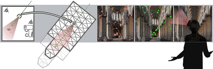
The inability to move decreases the level of immersion in the presented environment [ 61 ]. However, in order to make the comparison with the previously performed studies possible, the participants were not allowed to walk. For this reason, only stationary spherical images were used in the research (Fig.  2 ). The ratios, the location and the size of used details, materials, colors, contrasts, or intensity and angle at which the light is cast inside the interior were all identical to the ones used in the previous research. Just like then, three stimuli of varied nave length were generated. The ratios of the prepared visualizations were based on real buildings of this kind. The images were named as follows: A3D—cathedral with a short nave, B3D—cathedral with a medium-length nave, and C3D —cathedral with a long nave (Fig.  2 ).

Spherical visualizations and division into AOI. A3D—flattened spherical image prepared for the cathedral with a short nave, A3D spherical image for the cathedral with a short nave, which presents a part of the nave and the presbytery, B3D spherical image for the cathedral with a medium-length nave, C3D spherical image for the cathedral with a long nave, AOI INDICATORS—the manner of allocating and naming Areas of Interest. AOI names including the phrase 3D describe all elements not seen in the previous research. AOI names ending with 2D describe the elements shown in the previous research (Marta Rusnak on the basis of a visualization done by Wojciech Fikus).

Spherical images and flat images

The most striking difference between the two experiments is the scope of the image that the participants of the VR test were exposed to. The use of a spherical image made it possible to turn one’s head and look in all directions. Those who took part in the original test saw only a predetermined fragment of the interior. For the purpose of this study, this AOI was named “Research 2D”. The range of the architectural detail visible in the first test was marked with a red frame (Fig.  2 ). It might seem that the participants exposed to a flat image saw less than one-tenth of what the participants of the VR test were shown. This illusion stems from the nature of a flattened spherical image, which additionally enlarges the areas located close to the vantage point by strongly bending all nearby horizontal lines and surfaces. The same distortion is responsible for the fact that the originally square image here has a rounded top and bottom. An aspect where achieving homogeneous conditions proved difficult was the attempt to achieve the same balance of color, contrast and brightness on both the computer screen and the projector in the VR goggles. The settings—once deemed a satisfactory approximation of those applied in the original test – were not altered during the experiment.

The experiment, like the original research, included nine auxiliary images (Fig.  3 ). The presented material consisted of spherical photos taken inside churches in Wrocław, Poland. Each image, including the photos and the visualizations, was prepared so that the presbytery in each case would be located in the same spot, on the axis, in front of the viewer (Fig.  4 ).

Auxiliary images. a Church of the Virgin Mary on Piasek Island in Wrocław. b Church of Corpus Christi in Wrocław. c Church of St. Dorothy in Wrocław. d Dominican Church in Wrocław. e Czesław's Chapel in the Dominican Church in Wrocław. f Church of St. Maurice in Wrocław. g Church of St. Ignatius of Loyola in Wrocław h. Church of St. Michael the Archangel in Wrocław I Cathedral in Wrocław. (fot. MR)

Location of equipment in the lab. The idea was to maintain consistency between the lab space and the way spherical stimuli were presented.

Additional illustrations play an important role. Firstly, they made it possible to ensure that the studied interiors were not displayed when the participants behaved in an uncertain manner, unaware of how to execute the task at hand. Additionally, all photos showed the interior of churches. So, just like believers or tourists entering the temple, the participants were not surprised by the interior's function.

Just like in the previous research it was important to make it impossible for the participants to use their short-term memory while comparing churches with different lengths of nave, so each participant’s set of images included only one of the images under discussion (A3D—short or B3D—medium-length or C3D—long). Therefore three sets of stimuli had been prepared. The auxiliary images ensured randomness since the visualization A3D, B3D or C3D appeared as one of the last three stimuli. Each included instructional boards informing the participants about the rules of the experiment and allowing an individual calibration of the eye tracker, one of the three analyzed images and nine auxiliary images in the form of the aforementioned spherical photos. Analogically to the original experiment, the participants were given the same false task—they were supposed to identify those displayed buildings which, in their opinion, were located in Wrocław. This was meant to incite a homogeneous cognitive intention among the participants [ 62 ] when they looked at a new, uniquely unfamiliar interior. Since it was expected that the VR technology would be a fairly new experience for the majority of the participants, it was decided that the prepared visualizations would not be shown as one of the first three stimuli in a set. Other images were displayed in random order.

During that previous test, a trigger point function of the BeGaze (SMI) software was used, which allowed automatic display of an image once the participant looked at a specific predefined zone on the additional board. In Tobii ProLab [ 58 ] such a feature was not available. All visual stimuli were separated from one another by means of an additional spherical image. When participants looked at a red dot, the decision to display the next image had to be made by the person supervising the entire process.

The time span of registration that had been calculated for the original study was kept unchanged and amounted to 8 s. Unusual study time results from the experiment conducted in 2016 [ 14 ]. Comparisons are thus possible. However, this proved insufficient for the participants—5 out of 7 volunteers invited for preliminary tests and not included in the group undergoing analysis, expressed the need to spend more time looking at the images. It was suggested that the brevity of the display made the experience uncomfortable. Therefore the duration of a single display was increased to 16 s, but only the first eight were taken into consideration and used in the comparison.

Preparation of the room

Looking at a spherical image in VR did not allow movement within the displayed stimuli therefore the participants were asked to sit, just like in the study involving a stationary eye tracker. A change in the position of the participant’s body would require a change in the height of the camera and, as a result, a change in the perspective and that might have an adverse effect on the experiment. The room was quiet and dimming the light was possible. The positions of the participant’s seat and the VR base unit were marked on the room’s floor so as to make it possible to check and, if necessary, correct accidental shifts of the equipment (Fig.  4 ). It was important since any shifts in the position of the equipment would affect the orientation of the stimuli in space, making the direction in which the participant is initially looking inconsistent with the axes of the displayed interiors.

This section of the article describes the new results and then compares them to the previous observations of flat images.

Numerical data were generated using Tobii Pro Lab. Using the data from the registrations, collective numerical reports were prepared. Five main types of eye-tracking variables were analyzed: fixation count, visitors number, average fixation duration, total fixation duration, time to first fixation. Reports were generated automatically in Tobii Pro Lab. XLS files have been processed in Microsoft Excel and in Statistica 13.3. Graphs and diagrams were processed in PhotoShop CC2015.

In the end, biometric data was gathered correctly from 40 people who had been shown stimulus A3D, 40 people who had been shown stimulus B3D, and 37 people who had been shown stimulus C3D. That means that for various reasons 22% of registrations were deemed unusable for the purposes of the analysis (Fig.  1 ).

Due to the change in equipment and the environment of the experiment, more Areas of Interest were analyzed than during the previous study [ 35 ]. The way people looked at the spherical images was analyzed by dividing each of them into ten AOIs. Their location and names can be seen in Fig.  2 . In the frame located in the center one may find AOIs with a caption saying “2D”—that is because they correspond to the AOIs used in the flat images in the first study. All these AOIs can be summed up into one area named Old Research. Five more AOIs, which are placed over the parts of the image that had not been visible to those exposed to the flat stimuli, were captioned with names ending with “3D”.

Fixation report was done for the entire spherical image but also for the five old and five new research AOIs (Table 1 ). The number of fixations performed on entire stimuli A3D, B3D and C3D is not significantly different. Many more fixations were done on the Old Research AOI. The number of fixations performed within the five new AOIs decreased as the interior lengthened, whereas the values for the fields visible in the previous test increased.

To determine interest in particular parts of a stimulus, we can look at how many times those parts were viewed. Table 2 lists all 10 analyzed AOIs and their values. When viewing the data, it is important to consider the different numbers of participants who were shown the examples. Therefore the numbers are additionally shown as percentages. On inspection of the first part of the table it is apparent that the values presented in the five columns of new AOIs represent a decreasing trend.

With the extension of the interior proportions, three old AOIs gain more and more attention. The largest and most significant difference can be seen in the number of observers of the Vaults 2D AOI. For Floor 2D AOI, and Left Nave 2D AOI the number is decreasing, while the number of people looking at the Presbytery AOI is slightly increasing.

Another analyzed parameter is average fixation duration. Despite the noticed differences, the one-way ANOVA data analysis showed that all observed deviation in the fixation duration should be seen as statistically insignificant [ANOVA p > 0.05, due to the large number of groups compared, p values are placed in the Table 2 (line10 and 15)]. Despite this result, it is important that all three examples of the Presbytery 2D AOI have the longest-lasting fixations and for C3D the average fixation duration exceeded the value of 207 ms. This shows how visually important this AOI becomes for the interior with the longest nave.

The last generally analyzed feature is total visit duration. By far the largest difference in its value was recorded for the Vaults 2D AOI. Those exposed to stimulus C3D spent twice as much time looking at the vaults as did those exposed to stimulus AS. For the longest interior the attention time also increased for Right Nave 2D AOI, while the Floor 3D AOI shows almost no changes in visit duration. Data analysis shows that all observed deviations concerning average fixation duration and total visit duration are statistically insignificant (ANOVA F (2,117) / p > 0.05, exact values are in the Table 2 —line 10 and 15). This insignificance stems from the fact that the stimuli in question differ only slightly. The only thing that actually changes is the fragment of the main nave that is most distant from the observer. The data interpretation to follow is based on a general analysis of different aspects of visual behaviors and establishing increasing or decreasing tendencies between the AOIs for cases A3D, B3D and C3D. These observations are then juxtaposed with the relationships between stimuli observed in the 2D experiment. However, before engaging in a comparison, one needs to be certain that the cropped image chosen for the 2D experiment really consists of the area that those exposed to the interior looked at the longest.

One of the primary ideas behind doing research on the same topic again was to check the validity of the methodology used previously, including the author’s choice of how much of the interior was shown in the original stimuli. Should the participants of the VR experiment look for a very limited time at this area and instead find other parts of the building more attractive, it might suggest that some errors were made when making assumptions about either the previous research or the current one. In that case it would be impossible to make a credible comparison of the results obtained during those two experiments. A general analysis was therefore done for the Research 2D AOI. The value that perhaps best testifies to one’s cognitive engagement is the total visit duration calculated for all the AOIs visible in the previous research. The average value of this parameter amounted to 4.70 s, which is almost 59% of the registration span, for stimulus A3D; 4.14 s, which is 52% of registration span, for B3D; and 5.14 s, which is slightly over 64% of registration span, for C3D. What is interesting, an average of nearly ¾ of the participants’ fixations took place within the area presented in the previous research (70.1% to 75.9%) (Table 3 ).

That means that fixations within the Research 2D AOI were focused and that the participants made few fixations when looking to the sides or to the back. If those points of focus were more evenly distributed, one would be entitled to assume that no part of the interior drew attention in particular. However, these results suggest that the Research 2D AOI really did include the most important architectural elements in such a religious building as far as the impression made on an observer is concerned. This allows a further, more detailed analysis and comparison of the data obtained using a VR headset and those acquired by means of a stationary eye tracker.

Subsequent comparisons are made for single AOIs. In order to facilitate the comparison of the data gathered in both experiments, the names of the stimuli are expanded with distinctions of length: short cathedral A3D, medium-length cathedral B3D, long cathedral C3D. A graphic representation, which depicts all the AOIs for all three new spherical stimuli and three flat stimuli from old research, was prepared to allow a clear comparison of a large portion of numerical data. The upper part shows the schematics for the interior with a short nave (A2D and A3D), followed by the interiors with a medium-length nave (B2D and B3D), while the longest (C2D and C3D) are displayed at the bottom. Such graph was filled in with values corresponding to the given analyzed aspect: number of observers (Fig.  6 ), average fixation duration (Fig.  7 ), total visit duration (Fig.  8 ). Values inserted in the middle section were compared with the schemata shown above and below (Fig.  5 ). The range of the difference influenced the color-coding of the particular AOI, as determined in the attached legend. When the values were equal, the AOI was cream-colored. When the analysis showed a lower value, it was colored pink, and when an increase was noticed, it was colored green. Additional graphs, under described schemes, support the comparison.

The principle of color coding used in Figs.  6 , 7 and 8

Visitors count—omparison between three interiors short, medium and long nave . a 2D flat stimuli b 3D spherical stimuli. The charts c and d present only the data from the Old Research Area.

Average fixation duration—comparison between interiors with short, medium-length and long naves. a 2D flat stimuli, b 3D special stimuli. c A box plot—comparison between fixation duration for the entire three new and three old stimuli. Each box was drawn from Q1—first quartile to Q3—third quartile with a vertical line denoting the median. Whiskers indicate minimum and maximum. Outliers were sown as points ± 1.5 interquartile range.

Total visit duration—comparison between three interiors short, medium and long nave a 2D flat stimuli b 3D spherical stimuli. The charts ( c ) and ( d ) present only the data from the Research 2D Area.

The volunteers were able to make a series of movements looking up, down, to the back or to the sides. Changes in such activity may be analyzed by the number of people looking at particular AOIs. Figure  5 shows the combination of the three schemata and also includes the number of observers for each AOI. The upper part shows green coloring of most newly added AOIs in stimulus A3D. That suggests an increased movement of the participants. The 3D AOIs in the bottom part of the figure, which shows the data for stimulus C3D, is dominated with red color. It is very easy to notice the gradual decrease in the number of participants looking in other directions than forwards when comparing those exposed to stimuli A3D, B3D, and C3D. At this level of generalization the new study confirms previous findings. The vault and the presbytery, for example, were most willingly observed by people looking at interior C2D. One can easily notice that the number of those looking to the sides decreased along with an increase in the length of the nave. Many more people neglected looking at the Left Nave 3D AOI. It is plain to see that the longest nave discouraged the observers from looking to the sides of the spherical image.

People observing 2D images on a screen also looked sideways more when the church was shorter and less when its nave was lengthened. It has to be pointed out that there were relatively few of those who looked to the back of the spherical image. Here one could observe the same tendency as with looking to the sides—the longer the nave, the smaller the need to divert one’s gaze from the central part of the image. That is perhaps why not even one out of 37 people exposed to C3D looked at the back of the image during the 8 s that were recorded and analyzed. Similarly to the results of the previous research, the longer the nave became, the fewer people chose to look upwards at the Vaults 3D AOI. More people were inclined to look at the Vaults 2D AOI as the nave got shorter, which is visible in the visitors count.

Despite the differences in results obtained in the 2D and 3D experiments, the main tendencies proved not to be contradictory to each other as one may see in the graphs in Fig.  5 . It can be concluded that the most prominent deviation occurs in the Floor 3D AOI. It appears that the inability to look at other parts of the interior made the participants of the 2D study pay attention to the Floor AOI to a much greater extent. As the length of the nave grew, the attention paid to the Floor AOI decreased in both experiments. The deviations related to the other AOIs turned out to be not considerable. This seems particularly important in the case of the most important part of the interior—the presbytery. The author was afraid that the different nature of illustration switching (automatic in 2D versus manual in 3D) might adversely affect the number of participants looking at this AOI. However, nothing to that effect has been observed—the results for the Presbytery 2D AOI in both experiments are extremely similar.

Table 2 indicates that deviations in fixation duration are not statistically significant. Nevertheless, allowing a comparison of all fixations on all stimuli seems important (Fig.  7 ). Comparisons demonstrate many similarities between the 2D and 3D experiments.

In the 3D study the average duration of a single fixation within the Presbytery 2D AOI increases with the length of the nave. The duration of an average fixation for the Old Vaults AOI increases slightly as the nave gets longer. The same tendency was noticed in the research done on flat images even though the differences between the stimuli noticed in the current study were smaller in degree. In both cases visual magnetism of the vaults and the presbytery rises as they get further and further away from the observer.

A significant change should be noted in the average duration of a fixation for the entire image (A3D = 130 ms vs A2D = 290 ms, B3D = 136 ms vs B2D = 263 ms, C3D = 139 ms vs C2D = 271 ms). The average duration of fixations recorded for images displayed on the screen was twice as big as for those shown in the VR environment. A similar trend of shortening the duration of fixations from cognitive fixations (150–900 ms) into express fixations (90–150 ms) [ 63 ], although not as striking as in the research under discussion was noticed in VR by Gulhan et al. [ 54 ].

The comparison of the time the participants spent looking at individual AOIs in the 2D and 3D studies turned out to be very important. It allows one to clearly assess the impact of the way the interior is presented on how it is perceived (Fig.  8 ).

In the 2018 experiment the time the participants spent looking outside the screen would decrease along with the increase in the interior’s length. It was interpreted as a sign of boredom—the longer interior was slightly more complex and therefore kept the participants engaged for a longer period of time. In the 3D experiment those exposed to the stimulus with the medium-length and the longest nave respectively spent less and less time looking outside the Research 2D AOI. Such results, very similar in both experiments, allow one to state that the lengthening of the cathedral’s interior helps keep the interest of participants in the Presbytery 2D AOI and the areas closest to it.

Most AOIs have maintained a decreasing or increasing direction of change. However, one tendency was altered and seems contradictory to the hypothesis being verified. In the VR tests it turned out that the more distant—and therefore smaller—the presbytery was in the image, the less time on average the participants spent looking at it. This tendency could not be observed in the previous study.

Diagrams and graphs in Fig.  8 facilitate the comparison of the total visit duration results for the 2D and 3D tests. The diagram on the right shows more regularity. The analysis of the graphs show below makes it possible to see that there are two deviations in the graph on the left, of which the one related to the presbytery causes the most concern. In the case of the data from the VR recording, four out of five dependencies are regular. The scale of the irregularity related to the Left Nave 2D AOI in the VR experiment (bright blue line) is similar to the Right Nave 2D (dark blue line) in the 2D experiment. Large differences in the shape of the green and yellow lines in the charts (Fig.  8 c, d) that reflect how the total visit duration changed for the Floor 2D AOI and the Presbytery 2D AOI indicate that these two areas require analysis. The noticed deviations, in contrast to other AOI visible in both experiments, proved statistically significant (ANOVA, floor F (5,193)  = 38,29; p = 0.034/presbytery F (5,193)  = 78,21 p = 0.041). The attention paid to the floor is distinctly lower for all spherical stimuli, but decreases along with the increase in the length of the interior in both the 2D and 3D studies. On the other hand, the tendencies that characterize the visual attention paid to the presbytery in the flat-image research and in the research done on spherical images are visibly different. It is extremely interesting that astonishingly similar results were obtained for the Vaults 2D AOI (red lines).

In comparison to other eye-tracking tests mentioned in the introduction, the fact that useful data was obtained from 117 people is more than satisfactory. From a traditional point of view, the sample is small so the research has potentially low power, which minimizes the likelihood of reproducibility. This test also has a weakness of evaluating only three variations of one particular case study, which in addition is a computer-generated image and not a real-life interior. scientifically beneficial. Should one come up with such a three-part experiment, the methodology could be prepared with more precision and deliberation.

A similar experiment carried out on the basis of an actual interior and involving three different recording methods—stationary, mobile and VR eye tracking—would be very interesting and.

A different way of switching between successive stimuli in the 2D and 3D tests also may have affected the results of the comparison as far as the visual attention paid to the presbytery is concerned. Since in the 3D test it was not possible to establish field triggers that would automatically switch the images, one potential result is the lower number of fixations within the Presbytery 2D AOI. However, as evidenced by the comparison of the graphs in Fig.  6 , this difference in the switching method could not have had a major impact.

Despite using the same graphics program for both the 2D and 3D visualizations, the differences in the quality of the images displayed in two different environments in the two parts of the experiment may have influenced the results [ 64 ]. However, it must be considered as an element that cannot be separated from the chosen diagnostic tool. The construction of the VR goggles disturbs the assessment of distance regardless of the graphic quality of the displayed stimuli [ 65 ]. Unfamiliarity with the new technology may also create some minor difficulties as many people seem to find judging distances in VR difficult [ 66 , 67 ]. The fact that most deviations are not accidental and rather logically related to the previous test seems to suggest that the influence of this aspect on the research results was not significant.

Another element that might have influenced the results of the VR research was physical discomfort—mostly neck fatigue—connected with the weight of the device the participants put on their heads and observed in other cases of VR eye-tracking research [ 68 , 69 ]. However, the participants shown all three stimuli were equally exposed to this inconvenience, which makes it fairly impossible to affect the results and therefore the validity of the research.

The values discussed in the paper suggest that, even though a flat image is a major simplification of a real-life cognitive situation, the dominating reactions of the participants were sufficiently similar. Even though some differences can be observed, it is possible and justified to draw the same conclusion—the observers’ attention was directed much more effectively at the presbytery when the church’s interior was longer. Only three of the numerous analyzed features did not support the hypothesis of the existence of the longitudinal church effect. Even though the convergence is not perfect, it can be asserted that science confirms the genius of medieval thinkers and architects.

The amount of time the volunteers spent looking at the vaults did not change much between the two experiments. According to the comparative analysis, a shorter fixation time was observed in 3D. Fixation duration is usually regarded as an important indicator of visual engagement [ 70 ]. Aside from the examples of A2D and A3D, there were no significant differences in the number of observers who desired to view the vaults. 82% of participants observed vaults visible in A2D, while 50% of observers observed vaults in A3D (Fig.  6 ). This does not support the finding of Amanda Haskins’s team according to which an area attractive in a 2D experiment will prove even more attractive in 3D [ 56 ]. The results obtained in the research under discussion shows that AOIs that were visually attractive in the 2D test remained to a large extent equally attractive in the 3D test, whereas the AOIs that were less visually appealing in 2D, became even less appealing in 3D since the attention they would receive was divided between them and AOIs that did not exist in the 2D experiment. The fact that much larger deviations are noticed in 2D than in 3D suggests that it is preferable to study and discuss perception of architecture on the basis of 3D images or—should 2D need to be employed—using not one single flat image but several of its variations (just like three interiors of different length were used in this research) to facilitate more detailed and more precise comparison that in the end will result in more credible conclusions.

Conclusions

Despite the previously mentioned drawbacks and numerous doubts about research conducted with VR sets, the results obtained with spherical stimuli showed greater regularity than those collected during the 2D research. With the popularization and development of VR, some disadvantages of this technology are likely to diminish or disappear. Although 3D stimuli seem to be a better choice, the study does not assert that flat stimuli and stationary eye trackers should be abandoned as far as architectural research is concerned. The results of the comparative analysis also indicate that it is better not to derive conclusions from the data obtained from one single image but rather from a set of the given image’s slightly modified versions. If that is for some reason impossible, the absence of other values available for comparison makes evaluating and drawing correct conclusions fairly unreasonable. For this reason, it is advisable to use stationary eye tracking for research on issues related to cultural heritage that are less specific and more general.

The composition presented in the study has a simple, symmetrical layout with rhythmically repeating elements. In this way, a flat representation of the interior resulted in a reasonable interpretation of the results. It can be assumed that the more complex the composition to be analyzed with an eye tracker, the greater the impact of deviations resulting from the flat representation of the image.

Moreover, since the deviations in the gaze paths between a flat and spherical representation of the same faithfully modeled interior are easily noticeable, it seems obvious that they would be much greater should one use sketches, drawings or paintings instead of more real-life, photo-realistic stimuli. It appears only reasonable that implementation of such images would further distort the credibility of the obtained data and therefore they should not be employed in research on the visual perception of architecture or other tangible heritage. Studies that have had this form should be reviewed.

Data availability

The of datasets generated from 68 participants and analyzed during the current study are available in the RepOD repository. Marta Rusnak, Problem of 2D representation of 3D objects in architectural and heritage studies. Re-analysis of phenomenon of longitudinal church, RepOd V1; A lack of consent from all participants means other eye-tracking data are not publicly available. In line with the applicable legal and ethical principles, such a right belonged to volunteers. All graphic materials are included in the supplement. Study consent forms are preserved in the WUST archives.

Abbreviations

Eye-tracker

• Virtual reality

Augmented reality

Two dimensional

Three dimensional

Area of Interest

Dieckie G. Is psyhology relevant to aesthetics? Philos Rev. 1962;71:285–302. https://doi.org/10.2307/2183429 .

Article   Google Scholar  

Makin A. The gap between aesthetic science and aesthetic experience. Journal of Consciousness Studies 2017; 24 (1-2):184-213;

Zeki S, Bao Y, Pöppel E. Neuroaesthetics: the art, science, and brain triptych. Psych J. 2020;9:427–8. https://doi.org/10.1002/pchj.383 .

di Dio C, Vittorio G. Neuroaesthetics: a review. Curr Opin Neurobiol. 2009;19(6):682–7. https://doi.org/10.1016/j.conb.2009.09.001 .

Article   CAS   Google Scholar  

Poole A, Ball L. Eye tracking in human-computer interaction and usability research: current status and future prospects. In: Encyclopedia of human computer interaction. 2006. p. 211–9. https://doi.org/10.1016/B978-044451020-4/50031-1

Duchowski AT. Eye tracking methodology theory and practice. London: Springer-Verlag; 2007.

Google Scholar  

Holmqvist K, Nyström M, Andersson R, Dewhurst R, Jarodzka H, van de Weijer J. Eye tracking. A comprehensive guide to methods and measure. Oxford: Oxford University Press; 2011.

Michael I, Ramsoy T, Stephens M, Kotsi F. A study of unconscious emotional and cognitive responses to tourism images using a neuroscience method. J Islam Mark. 2019;10(2):543–64. https://doi.org/10.1108/JIMA-09-2017-0098 .

Dalby Kristiansen E, Rasmussen G. Eye-tracking recordings as data in EMCA studies: exploring possibilities and limitations. Social Interact Video-Based Studies Hu Social. 2021. https://doi.org/10.7146/si.v4i4.121776 .

Graham J, North LA, Huijbens EH. Using mobile eye-tracking to inform the development of nature tourism destinations in Iceland. In: Rainoldi M, Jooss M, editors. Eye Tracking in Tourism. Cham: Springer International Publishing; 2020. p. 201–24.

Chapter   Google Scholar  

Han E. Integrating mobile eye-tracking and VSLAM for recording spatial gaze in works of art and architecture. Technol Arch Design. 2021;5(2):177–87. https://doi.org/10.1080/24751448.2021.1967058 .

Chadalavada RT, Andreasson H, Schindler M, Palm R, Lilienthal AJ. Bi-directional navigation intent communication using spatial augmented reality and eye-tracking glasses for improved safety in human–robot interaction. Robo Computer-Integrated Manufact. 2020;61: 101830. https://doi.org/10.1016/j.rcim.2019.101830 .

Campanaro DM, Landeschi G. Re-viewing Pompeian domestic space through combined virtual reality-based eye tracking and 3D GIS. Antiquity. 2022;96:479–86.

Rusnak M, Fikus W, Szewczyk J. How do observers perceive the depth of a Gothic cathedral interior along with the change of its proportions? Eye tracking survey. Architectus. 2018;53:77–88.

Francuz P. Imagia. Towards a neurocognitive image theory. Lublin: Katolicki Uniwersytet Lubelski; 2019.

Walker F, Bucker B, Anderson N, Schreij D, Theeuwes J. Looking at paintings in the Vincent Van Gogh Museum: eye movement patterns of children and adults. PLoS ONE. 2017. https://doi.org/10.1371/journal.pone.0178912 .

Mitrovic A, Hegelmaier LM, Leder H, Pelowski M. Does beauty capture the eye, even if it’s not (overtly) adaptive? A comparative eye-tracking study of spontaneous attention and visual preference with VAST abstract art. Acta Physiol (Oxf). 2020;1(209): 103133. https://doi.org/10.1016/j.actpsy.2020.103133 .

Jankowski T, Francuz P, Oleś P, Chmielnicka-Kuter E, Augustynowicz P. The Effect of painting beauty on eye movements. Adv Cogn Psychol. 2020;16(3):213–27. https://doi.org/10.5709/acp-0298-4 .

Ferretti G, Marchi F. Visual attention in pictorial perception. Synthese. 2021;199(1):2077–101. https://doi.org/10.1007/s11229-020-02873-z .

Coburn A, Vartanian O, Chatterjee A. Buildings, beauty, and the brain: a neuroscience of architectural experience. J Cogn Neurosci. 2017;29(9):1521–31. https://doi.org/10.1162/jocn_a_01146 .

Al-Showarah S, Al-Jawad N, Sellahewa H. Effects of user age on smartphone and tablet use, measured with an eye-tracker via fixation duration, scan-path duration, and saccades proportion. In: Al-Showarah S, Al-Jawad N, Sellahewa H, editors. Universal access in human-computer interaction universal access to information and knowledge: 8th international conference, UAHCI 2014, Held as Part of HCI International 2014, Heraklion, Crete, Greece, June 22-27, 2014, Proceedings, Part II. Cham: Springer; 2014. p. 3–14.

Todorović D. Geometric and perceptual effects of the location of the observer vantage point for linear-perspective images. Perception. 2005;34(5):521–44. https://doi.org/10.1068/p5225 .

Itti L, Koch C. Computational modelling of visual attention. Nat Rev Neurosci. 2001;2(3):194–203. https://doi.org/10.1038/35058500 .

Redi J, Liu H, Zunino R, Heynderickx I. Interactions of visual attention and quality perception. ProcSPIE. 2011. https://doi.org/10.1117/12.876712 .

Rusnak M. Eye-tracking support for architects, conservators, and museologists. Anastylosis as pretext for research and discussion. Herit Sci. 2021;9(1):81. https://doi.org/10.1186/s40494-021-00548-7 .

Clay V, König P, König SU. Eye tracking in virtual reality. J Eye Mov Res. 2019. https://doi.org/10.16910/jemr.12.1.3 .

Brielmann AA, Buras NH, Salingaros NA, Taylor RP. What happens in your brain when you walk down the street? implications of architectural proportions, biophilia, and fractal geometry for urban science. Urban Sci. 2022; 6(1):3  https://doi.org/10.3390/urbansci6010003 .

Böhme G. Atmospheric architectures: the aesthetics of felt spaces brings. Engels-Schwarzpaul T, editor. London, Oxford, New York: Bloomsbury; 2017.

Panofsky E. Architecture gothique et pensée scolastique précédé de L’abbé Suger de Saint-Denis, Les Edition de Minuit, Alençon . Alençon : Les Edition de Minuit; 1992.

Henry-Claude M. SL, ZY,. Henry-Claude M., Stefanon L., Zaballos Y., Principes et éléments de l’architecture religieuse médievale, . Gavaudun : Fragile; 1997.

Scot RA. The Gothic Enterprise. Guide to understand the Medieval Cethedral. California: University of California Press; 2003.

Erlande-Brandenburg A. MBAB,. Histoire de l’architecture Française. Du moyen Age à la Reinaissance: IVe siècle–début XVIe siècle, Caisse nationale des monuments historiques et des sites. Paris : Mengès; 1995.

Norman E. The house of god. Goring by the sea, Sussex: Thames & Hudson; 1978.

Duby G, Levieux E. The age of the cathedrals: art and society, 980–1420. Chicago: University of Chicago Press; 1983.

Rusnak M, Chmielewski P, Szewczyk J. Changes in the perception of a presbytery with a different nave length: funnel church in eye tracking research. Architectus. 2019;2:73–83.

Zhang L, Jeng T, Zhang RX. Integration of virtual reality, 3-D eye-tracking, and protocol analysis for re-designing street space. In: Alhadidi S, Crolla K, Huang W, Janssen P, Fukuda T, editors. CAADRIA 2018 - 23rd international conference on computer-aided architectural design research in Asia learning, prototyping and adapting. 2018.

Zhang RX, Zhang LM. Panoramic visual perception and identification of architectural cityscape elements in a virtual-reality environment. Futur Gener Comput Syst. 2021;118:107–17. https://doi.org/10.1016/j.future.2020.12.022 .

Crucq A. Viewing patterns and perspectival paintings: an eye-tracking study on the effect of the vanishing point. J Eye Mov Res. 2021. https://doi.org/10.16910/jemr.13.2.15 .

Raffi F. Full Access to Cultural Spaces (FACS): mapping and evaluating museum access services using mobile eye-tracking technology. Ars Aeterna. 2017;9:18–38. https://doi.org/10.1515/aa-2017-0007 .

Mokatren M, Kuflik T, Shimshoni I. Exploring the potential of a mobile eye tracker as an intuitive indoor pointing device: a case study in cultural heritage. Futur Gener Comput Syst. 2018;81:528–41. https://doi.org/10.1016/j.future.2017.07.007 .

Jung YJ, Zimmerman HT, Pérez-Edgar K. A methodological case study with mobile eye-tracking of child interaction in a science museum. TechTrends. 2018;62(5):509–17. https://doi.org/10.1007/s11528-018-0310-9 .

Reitstätter L, Brinkmann H, Santini T, Specker E, Dare Z, Bakondi F, et al. The display makes a difference a mobile eye tracking study on the perception of art before and after a museum’s rearrangement. J Eye Mov Res. 2020. https://doi.org/10.16910/jemr.13.2.6 .

Rusnak M, Szewczyk J. Eye tracker as innovative conservation tool. Ideas for expanding range of research related to architectural and urban heritage. J Herit Conserv. 2018;54:25–35.

de la Fuente Suárez LA. Subjective experience and visual attention to a historic building: a real-world eye-tracking study. Front Architect Res. 2020;9(4):774–804. https://doi.org/10.1016/j.foar.2020.07.006 .

Rusnak M, Ramus E. With an eye tracker at the Warsaw Rising Museum: valorization of adaptation of historical interiors. J Herit Conserv. 2019;58:78–90.

Junker D, Nollen Ch. Mobile eyetracking in landscape architecture. Analysing behaviours and interactions in natural environments by the use of innovative visualizations. In: Proceeding of the international conference “Between Data and Science” Architecture, neuroscience and the digital worlds. 2017.

Kabaja B, Krupa M. Possibilities of using the eye tracking method for research on the historic architectonic space in the context of its perception by users (on the example of Rabka-Zdrój). Part 1. Preliminary remarks. J Herit Conserv. 2017;52:74–85.

Kiefer P, Giannopoulos I, Kremer D, Schlieder C, Martin R. Starting to get bored: An outdoor eye tracking study of tourists exploring a city. In: Eye Tracking Research and Applications Symposium (ETRA). 2014.

Karakas T, Yildiz D. Exploring the influence of the built environment on human experience through a neuroscience approach: a systematic review. Front Archit Res. 2020;9(1):236–47. https://doi.org/10.1016/j.foar.2019.10.005 .

Mohammadpour A, Karan E, Asadi S, Rothrock L. Measuring end-user satisfaction in the design of building projects using eye-tracking technology. Austin, Texas: American Society of Civil Engineers; 2015.

Book   Google Scholar  

Dupont L, Ooms K, Duchowski AT, Antrop M, van Eetvelde V. Investigating the visual exploration of the rural-urban gradient using eye-tracking. Spat Cogn Comput. 2017;17(1–2):65–88. https://doi.org/10.1080/13875868.2016.1226837 .

Holmqvist K, Nyström M, Mulvey F. Eye tracker data quality: what it is and how to measure it. in: proceedings of the symposium on eye tracking research and applications. New York. Association for computing machinery; 2012. p. 45–52. (ETRA ’12). https://doi.org/10.1145/2168556.2168563

Foulsham T, Walker E, Kingstone A. The where, what and when of gaze allocation in the lab and the natural environment. Vision Res. 2011;51(17):1920–31. https://doi.org/10.1016/j.visres.2011.07.002 .

Gulhan D, Durant S, Zanker JM. Similarity of gaze patterns across physical and virtual versions of an installation artwork. Sci Rep. 2021;11(1):18913. https://doi.org/10.1038/s41598-021-91904-x .

van Herpen E, van den Broek E, van Trijp HCM, Yu T. Can a virtual supermarket bring realism into the lab? Comparing shopping behavior using virtual and pictorial store representations to behavior in a physical Store. Appetite; 2016;107,196-207.  https://doi.org/10.1016/j.appet.2016.07.033 .

Haskins AJ, Mentch J, Botch TL, Robertson CE. Active vision in immersive, 360° real-world environments. Sci Rep. 2020;10: art. nr 14304. https://doi.org/10.1038/s41598-020-71125-4 .

Hayhoe MM, Shrivastava A, Mruczek R, Pelz JB. Visual memory and motor planning in a natural task. J Vis. 2003;3(1):49–63. https://doi.org/10.1167/3.1.6 .

https://www.tobiipro.com/ . (accessed 10.05.2022)

Francuz P, Zaniewski I, Augustynowicz P, Kopí N, Jankowski T, Jacobs AM, et al. Eye movement correlates of expertise in visual arts. Front Hum Neurosci. 2018;12:87. https://doi.org/10.3389/fnhum.2018.00087 .

Koide N, Kubo T, Nishida S, Shibata T, Ikeda K. Art Expertise reduces influence of visual salience on fixation in viewing abstract-paintings. PLoS ONE. 2015;10(2): e0117696. https://doi.org/10.1371/journal.pone.0117696 .

Pangilinan E, LS& M v. Creating augmented and virtual realities: theory and practice for next-generation spatial computing. sebastopol: O’Reilly Media; 2019.

Tatler BW, Wade NJ, Kwan H, Findlay JM, Velichkovsky BM. Yarbus, eye movements, and vision. Iperception. 2010;1(1):382.

Galley N, Betz D, Biniossek C. Fixation durations—why are they so highly variable? . In: Advances in visual perception research. Thomas Heinen. Hildesheim: Nova Biomedicaal; 2015. p. 83–106.

Stevenson N, Guo K. Image valence modulates the processing of low-resolution affective natural scenes. Perception. 2020;49(10):1057–68. https://doi.org/10.1177/0301006620957213 .

Thompson WB, Willemsen P, Gooch AA, Creem-Regehr SH, Loomis JM, Beall AC. Does the quality of the computer graphics matter when judging distances in visually immersive environments? Presence Teleoperators Virtual Environ. 2004;13(5):560–71. https://doi.org/10.1162/1054746042545292 .

Choudhary Z, Gottsacker M, Kim K, Schubert R, Stefanucci J, Bruder G, et al. Revisiting distance perception with scaled embodied cues in social virtual reality. In: Proceedings—2021 IEEE Conference on Virtual Reality and 3D User Interfaces, VR 2021. 2021. p. 788–97. https://doi.org/10.1109/VR50410.2021.00106

Jamiy FE, Ramaseri CAN, Marsh R. Distance accuracy of real environments in virtual reality head-mounted displays. In: 2020 IEEE international conference on electro information technology (EIT). 2020. p. 281–7. https://doi.org/10.1109/EIT48999.2020.9208300

McGill M, Kehoe A, Freeman E, Brewster SA. Expanding the bounds of seated virtual workspaces. ACM Trans Comput-Hum Interact (TOCHI). 2020;27:1–40. https://doi.org/10.1145/3380959 .

Mon-Williams M, Plooy A, Burgess-Limerick R, Wann J. Gaze angle: a possible mechanism of visual stress in virtual reality headsets. Ergonomics. 1998;41(3):280–5. https://doi.org/10.1080/001401398187035 .

Nuthmann A, Smith T, Engbert R, Henderson J. CRISP: a computational model of fixation durations in scene viewing. Psychol Rev. 2010;117(2):382–405. https://doi.org/10.1037/a0018924 .

Download references

Acknowledgements

Cooperation: Hardware consultation: Ewa Ramus (Neuro Device, Warszawa, Poland), graphic cooperation: Wojciech Fikus (Wroclaw University of Science and Technology, Poland), data collecting: Mateusz Rabiega (Wroclaw University of Science and Technology, Poland), Magdalena Nawrocka (Wroclaw University of Science and Technology, Poland), Małgorzata Cieślik (independent, Wrocław, Poland), Daria Kruczek (independent, London, UK). The author would like to thank Ewa Ramus, Neuro Device and the technology company Tobii for the opportunity to develop an initial prototype of VR eye-tracking implementation. It is worth mentioning the support of Andrzej Żak. Thank you Marcin!

Human participation statement: WUST Ethical Committee approved the experiments and its protocols. Informed consent was obtained from all participants.

This work was supported by the National Science Center, Poland (NCN) under Miniatura Grant [2021/05/X/ST8/00595].

Author information

Authors and affiliations.

Wrocław University of Science and Technology, Bolesława Prusa 53/55, 53-317, Wrocław, Poland

Marta Rusnak

You can also search for this author in PubMed   Google Scholar

Contributions

MR- methodology, experiment design, data acquisition and analysis, writing. Author read and approved the final manuscript.

Corresponding author

Correspondence to Marta Rusnak .

Ethics declarations

Competing interests.

The author declares no competing interests.

Additional information

Publisher's note.

Springer Nature remains neutral with regard to jurisdictional claims in published maps and institutional affiliations.

Rights and permissions

Open Access This article is licensed under a Creative Commons Attribution 4.0 International License, which permits use, sharing, adaptation, distribution and reproduction in any medium or format, as long as you give appropriate credit to the original author(s) and the source, provide a link to the Creative Commons licence, and indicate if changes were made. The images or other third party material in this article are included in the article's Creative Commons licence, unless indicated otherwise in a credit line to the material. If material is not included in the article's Creative Commons licence and your intended use is not permitted by statutory regulation or exceeds the permitted use, you will need to obtain permission directly from the copyright holder. To view a copy of this licence, visit http://creativecommons.org/licenses/by/4.0/ . The Creative Commons Public Domain Dedication waiver ( http://creativecommons.org/publicdomain/zero/1.0/ ) applies to the data made available in this article, unless otherwise stated in a credit line to the data.

Reprints and permissions

About this article

Cite this article.

Rusnak, M. 2D and 3D representation of objects in architectural and heritage studies: in search of gaze pattern similarities. Herit Sci 10 , 86 (2022). https://doi.org/10.1186/s40494-022-00728-z

Download citation

Received : 28 April 2022

Accepted : 01 June 2022

Published : 16 June 2022

DOI : https://doi.org/10.1186/s40494-022-00728-z

Share this article

Anyone you share the following link with will be able to read this content:

Sorry, a shareable link is not currently available for this article.

Provided by the Springer Nature SharedIt content-sharing initiative

• Eye tracker
• Methodology
• Flat and spherical stimulus

Thank you for visiting nature.com. You are using a browser version with limited support for CSS. To obtain the best experience, we recommend you use a more up to date browser (or turn off compatibility mode in Internet Explorer). In the meantime, to ensure continued support, we are displaying the site without styles and JavaScript.

• View all journals
• My Account Login
• Explore content
• About the journal
• Publish with us
• Sign up for alerts
• Open access
• Published: 29 May 2024

The impact of presentation modes on mental rotation processing: a comparative analysis of eye movements and performance

• Philipp Stark 1 ,
• Efe Bozkir 3 , 4 ,
• Weronika Sójka 1 ,
• Markus Huff 2 , 5 ,
• Enkelejda Kasneci 4 &
• Richard Göllner 1 , 6  

Scientific Reports volume  14 , Article number:  12329 ( 2024 ) Cite this article

86 Accesses

1 Altmetric

Metrics details

• Human behaviour

Mental rotation is the ability to rotate mental representations of objects in space. Shepard and Metzler’s shape-matching tasks, frequently used to test mental rotation, involve presenting pictorial representations of 3D objects. This stimulus material has raised questions regarding the ecological validity of the test for mental rotation with actual visual 3D objects. To systematically investigate differences in mental rotation with pictorial and visual stimuli, we compared data of \(N=54\) university students from a virtual reality experiment. Comparing both conditions within subjects, we found higher accuracy and faster reaction times for 3D visual figures. We expected eye tracking to reveal differences in participants’ stimulus processing and mental rotation strategies induced by the visual differences. We statistically compared fixations (locations), saccades (directions), pupil changes, and head movements. Supplementary Shapley values of a Gradient Boosting Decision Tree algorithm were analyzed, which correctly classified the two conditions using eye and head movements. The results indicated that with visual 3D figures, the encoding of spatial information was less demanding, and participants may have used egocentric transformations and perspective changes. Moreover, participants showed eye movements associated with more holistic processing for visual 3D figures and more piecemeal processing for pictorial 2D figures.

Similar content being viewed by others

Randomness impacts the building of specific priors, visual exploration, and perception in object recognition

Processing of translational, radial and rotational optic flow in older adults

Assessing the allocation of attention during visual search using digit-tracking, a calibration-free alternative to eye tracking

Introduction.

Mental rotation, the ability to rotate mental representations of objects in space, is a core ability for spatial thinking and spatial reasoning 1 , 2 . Mental rotation is required for everyday skills, like map reading or navigating, and is an important prerequisite for individuals’ learning 3 . Higher mental rotation performance is associated with higher fluid intelligence and better mathematical thinking 4 . It has been found to be beneficial for students’ learning in mathematics domains such as geometry and algebra 5 . Thus, mental rotation ability acts as a gatekeeper for entering STEM-related fields in higher education 6 .

A standardized test by Shepard and Metzler 7 for measuring humans’ mental rotation performance displays two-dimensional (2D) images of two unfamiliar three-dimensional (3D) figures. For these pictorial stimuli, participants are instructed to determine whether the two figures are identical. For this, the two figures are depicted from different perspectives by independently rotating one of them along its axis 7 , 8 . Individuals’ performance in mental rotation is reflected by the number of correct answers and task-solving speed (reaction time) 9 , 10 . Since its initial development, this experiment has been replicated many times 10 , 11 , 12 , 13 . The test by Shepard and Metzler is one of the most frequently used tests to examine mental rotation. It laid the foundation for understanding spatial cognition 14 , 15 , 16 , 17 and continues to be referenced in contemporary research 10 , 18 , 19 . Replicating this classic experiment allows researchers to build on a well-established foundation and examine enduring principles of mental rotation.

However, its ecological validity to assess real-life mental rotation has been questioned 20 , 21 . Developments in the field of virtual simulations enable experiments to be conducted with increased ecological validity yet still under controlled and standardized conditions 22 . In particular, virtual realities (VR) have become powerful tools in psychological research 23 , 24 . VR allows for the creation of environments with 3D spatial relations that can be explored and manipulated by users and are experienced in an immersive way 25 . This allows for the presentation of visual 3D figures, rendered as 3D objects in the environment, and introduces visual and perceptual differences to pictorial (2D) stimuli.

The pictorial stimuli of the conventional mental rotation test are orthographic, parallel representations of 3D figures on a planar surface (as images). This pictorial representation lacks two sources of depth information present in visual (3D) figures when placed in a VR environment with realistic spatial relations 26 . The first source of depth information is provided by stereoscopic vision due to binocular disparity. The binocular disparity stems from the slight offset between the two displays projected onto the two eyes in the head-mounted display (HMD), enabling stereopsis and depth perception 27 . This depth cue is particularly relevant for 3D vision, where it contributes to participants’ ability to perceive depth and spatial relationships between objects. The second source of depth information is introduced by motion parallax 26 , 28 . Motion parallax, also known as structure-from-motion, emerges as a consequence of real-time head tracking and rendering based on the observer’s position within the virtual space. This dynamic depth cue allows users to perceive the 3D structure of objects by moving their heads. As they move relative to the 3D object, the representation of the object is updated and provides different views to identify the object. Furthermore, shadows provide additional depth information. They occur when physical objects interact with light sources in a VR environment. Shadows contribute to the perception of object volume and spatial relationships in visual figures. Presenting mental rotation stimuli in VR provides the most comprehensive visual information. In contrast, rear-projection systems offer solely pictorial information 29 , and stereoscopic glasses introduce binocular disparity 30 , leaving motion parallax as the final piece of the puzzle added by VR 31 .

This additional visual information is expected to affect participants’ stimulus processing and mental rotation strategy when solving items with visual stimuli in comparison to pictorial representations. A series of processing steps when solving mental rotation tasks have been identified 32 , 33 : (1) encoding and searching, which combines the perceptual encoding of the stimulus and the identification of the stimulus and its orientation; (2) transformation and comparison, which includes the actual process of mentally rotating objects; (3) judgment and response, which combines the confirmation of a match or mismatch between the stimuli and the response behavior.

One would expect the visual modes of presentation to introduce differences in the processing steps. During encoding and searching with pictorial figures, a model of the 3D object structure must be recovered from a planar 2D representation 34 . This reconstruction process has been found to be a demanding task 35 and should not be necessary with visual figures. One would also expect the identification of the stimulus and its orientation to be more demanding with pictorial figures. A displayed image remains static regardless of the observer’s location; therefore, participants have to make assumptions about occluded or ambiguous parts of the figure. For pictorial figures, the additional head movement might even produce perceptual distortions described by the differential rotation effect 36 , in which the size and shape of images are perceived inappropriately when the observer is not in the center of the projection 37 . In contrast, binocular disparity and motion parallax would constantly update the visual 3D figures based on the participants’ relative location to the object. Test takers can explore the visual figures and gather additional information from different perspectives, which should help them to identify the figures and their orientation more easily.

In the second step of transformation and comparison, mental rotation involves manipulating and rotating mental representations of geometric figures in the mind. Exploiting motion parallax with visual 3D figures could reduce the need for extensive mental transformations. For example, participants could reduce the rotation angle between the figures through lateral head movement. The rotation angle is the degree to which the figures are rotated against each other. This may make the comparison process more intuitive and less cognitively demanding. Motion parallax due to head movement could also lead to a shift from the object-based transformation of the stimuli to an egocentric transformation 38 . In object-based transformations, the observer’s position remains fixed while the object is mentally rotated. An egocentric transformation involves a change of perspective, rotating one’s body to change the viewpoint and orientation. It has been found that egocentric transformations, as a form of self-motion, are more intuitive and result in faster and more accurate mental rotation 39 .

Similar reaction times for mental and manual rotation suggest that participants mentally align the figures to each other for comparison 40 . Two prominent alignment strategies have been described for mental rotation: piecemeal and holistic. The piecemeal strategy involves breaking down the object into segments and mentally rotating the pieces in congruence with the comparison object to assess their match. A holistic approach entails mentally rotating the entire object and encoding comprehensive spatial information about it 41 , 42 . In their original study, Shepard and Metzler viewed the linear relationship between rotation angle and reaction time as evidence against conceptual or propositional processing of visual information 7 , 43 . Later research, which investigated the process of rotation itself, revealed that both a holistic and a piecemeal approach were used to align the figures 16 , 42 , 44 . When processing visual figures, motion parallax allows for lateral head movements, which could be used to decrease the rotation angle between the figures by changing perspectives. The additional depth information due to binocular disparity could facilitate the comparison of spatial relationships between object features. These aspects might enable a more holistic processing of the figures.

Regarding judgment and response, participants are expected to perform better with visual 3D figures than with pictorial 2D figures. Lower cognitive demands during encoding might result in faster stimulus processing. The potential to apply an egocentric transformation and more holistic processing can be expected to lead to more efficient and more accurate responses with visual 3D figures.

The process of mental rotation is reflected in eye movements, which capture the visual encoding of spatial information 13 , 33 . Eye movement metrics can provide comprehensive information on stimulus processing and mental rotation strategies 13 , 41 , 42 , 45 , 46 , 47 . Basic experiments have shown that eye movements are controlled by cognitive processes, and consequently, it is possible to distinguish task-specific processes 48 . For example, different mental rotation strategies were identified and discriminated based on fixation patterns derived from eye-tracking data 16 . Fixation measures that incorporate spatial information are expected to reveal relevant information about stimulus processing. Different fixations on different segments of the figures have been associated with the first or second processing steps 33 . During the step of encoding and searching, the majority of fixations targeted one segment of one figure, whereas in the second step of transformation and comparison, fixations targeted all segments of both figures equally. This should lead to a higher fixation duration on singular segments in the first step and an equal fixation duration on all parts of the figure in the second step.

Saccadic movements between fixations, measured by saccade rate or saccade velocity, have also been utilized to investigate mental rotation with pictorial figures 33 , 46 , 49 . Directional saccadic movements containing spatial information can reveal temporal dependencies in stimulus processing 33 . For example, a backward saccade that guides the eye toward a previous location is called a regressive saccade 50 . We would expect that the regression towards a previous location could either be a need for information retrieval of figure information or a back-and-forth between congruent figure segments during the comparison step.

Regarding mental rotation strategies, information about the number of transitions between figures compared to the number of fixations within the figures has been applied to quantify the use of holistic vs. piecemeal strategies 42 , 46 . The ratio of the number of within-object fixations divided by the number of between-objects fixations has been shown to indicate holistic processing (ratio \(\le 1\) ) or piecemeal processing (ratio \(> 1\) ) 42 , 51 .

The pupil diameter provides information about the size of the pupil in both eyes and can be used to detect changes due to contraction and dilation. An increase in pupil diameter has been associated with higher cognitive load 52 , 53 , 54 , as the Locus Coeruleus (LC) controls pupil dilation and is engaged in memory retrieval 55 , 56 . Moreover, two different measures of pupil diameter behavior have been attributed to the phasic and tonic modes of LC activity 55 . Tonic mode activity is indicated by a larger overall pupil diameter and is associated with lower task utility and higher task difficulty. Phasic mode activity is indicated by larger pupil size variation during the task and is associated with task engagement and task exploitation 13 , 57 . While solving mental rotation tasks, a larger average pupil diameter over individual trials could indicate tonic activity, whereas a larger peak pupil diameter as a task-evoked pupillary response could indicate phasic activity 13 , 56 .

Recently available devices for analyzing eye movements in VR experiments include eye-tracking apparatuses. These devices record sensory data frame by frame to track visual and sensorimotor information in a standardized way during experiments 58 . The VR’s HMD additionally allows for tracking head movement. Changes in head movement serve as a valuable indicator of whether participants make use of motion parallax. A recently published study by Tang et al. 46 analyzed eye movements during a mental rotation task in VR, but solely for visual 3D figures. The results of their VR experiment showed that the mental rotation test with visual 3D figures replicates the linear relationship between rotation angle and reaction time. Lochhead et al. 31 , on the other hand, investigated performance differences between pictorial and visual 3D figures presented in VR. Their results indicated that participants exhibited higher performance in the 3D condition compared to the 2D condition. However, they did not use eye tracking to capture participants’ visual processing of the stimuli to potentially explain presentation mode effects on performance.

Our study used a VR laboratory (see Fig.  2 ) to examine individuals’ mental rotation performance for pictorial 2D figures and visual 3D figures with the Shepard and Metzler test. We examined eye and head movements from \(N = 54\) university student participants to determine differences in stimulus processing and mental rotation strategies when solving mental rotations with pictorial and visual stimuli. In both conditions, 28 stimuli pairs were shown, modeled after the original figures by Shepard and Metzler 7 . In the 3D condition, stimuli were rendered on a virtual table in front of the participants, allowing them to view the figures from different perspectives by moving their heads. In the 2D condition, the stimuli appeared on a virtual screen placed on the table at the same distance from the participants as in the 3D conditions. A series of 3D and 2D figures were presented, with the two conditions randomized block-wise within each student. For each task, participants’ performance in terms of the number of correct answers and reaction time as well as eye-movement features were recorded. The following hypotheses were formulated:

First, we expected participants’ performance in solving mental rotation tasks to be better with visual 3D figures than with pictorial 2D figures. Second, we expected the visual differences to evoke differences in stimulus processing and mental rotation strategies, which may indicate differences in performance between the two modes of presentation. To investigate this hypothesis, we analyzed how eye and head movements differed during task-solving in both conditions. To ensure that we could compare all stimulus pairs between the two conditions, no overall time limit was set for the experiment.

In addition to utilizing statistical analysis, we implemented a Gradient Boosting Decision Tree (GBDT) 59 classification algorithm to identify the experimental condition based on eye and head movements. This machine learning approach surpassed traditional linear statistical methods, which are often limited to linear relationships between features and the target variable. Successfully predicting the experiment condition based on eye and head movement features would demonstrate the importance of these features for the distinguishing task.

Behavioral data, such as eye and head movements, are characterized by temporal dependencies and determined by biological mechanisms (e.g., a fixation is followed by a saccade and vice versa), which often results in high collinearity between the features 60 . From the class of machine learning models, we selected GBDT rather than other models like Support Vector Machines or Random Forest because of its ensemble approach. Ensemble methods can handle some degree of collinearity by partitioning the feature space into separate regions 61 . Previous research has demonstrated the suitability of GBDT models for spatial reasoning tasks involving geometrical objects, which are comparable to the task utilized in this study 62 .

Provided that the GBDT model classifies the conditions correctly, a Shapley Additive Explanations (SHAP) explainability approach can be applied 63 . The SHAP approach provides information on both global and local feature importance. Global feature importance ranks input features by their significance for accurate model predictions, identifying the most relevant features for differentiating between the experimental conditions. Local feature importance supplements this by providing additional information on the relationship between feature variables and target variables. It reveals which feature values were attributed to each condition and how effectively those values distinguish between conditions. These aspects complement statistical analyses and offer valuable insights into the relationship between eye movements and mental rotation processing.

Mental rotation performance differences

All participants completed both experimental conditions (2D and 3D) in a block-wise randomized condition order. The mean values and standard deviations of all variables in each condition are depicted in Table  1 . Further information about the distributions is presented in Supplementary Table S1 . We used a non-parametric, paired Wilcoxon signed-rank test since some variables were not normally distributed. We report the Z statistics from two-tailed, paired tests with p values. Additionally, we applied a two-tailed, paired t-test and compared the results for skewed distributions (Supplementary Table S2 ).

On average, participants spent 11.91 min in VR ( \(SD=3.65\;min\) ) without any breaks in between. In the 2D condition, participants solved \(83.2\%\) of the stimuli correctly on average ( \(M=0.832\) , \(SD= 0.105\) ), while in the 3D condition, they solved \(88.2\%\) correctly ( \(M=0.882\) , \(SD=0.101\) ). Participants achieved a significantly higher percentage of correct answers in the 3D condition ( \(Z=243\) , \(p=.001\) ) when comparing the 2D with the 3D condition in a two-tailed test. Participants exhibited a longer reaction time (in seconds, \(M=6.861\) , \(SD=3.583\) ) in the 2D condition than in the 3D condition ( \(M=6.076\) , \(SD=3.214\) ). Based on a two-tailed test, reaction time differed significantly between the conditions ( \(Z=1168\) , \(p<0.001\) ). Details of the statistical analysis are shown in Table  2 .

To ensure that the differences in performance could not be attributed to sex differences, we performed additional statistical analyses to verify this. No sex differences were found in our study. This is consistent with previous research, which reported no sex differences in experiments conducted without time constraints 12 , 18 or using less abstract stimulus materials 13 , 64 . Detailed statistics can be found in Supplementary Table S3 .

We verified that the performance differences between 2D and 3D are not attributed to order effects. The average reaction time was always found to be higher in the 2D condition, regardless of the order. However, the differences were larger when the 2D condition was presented first. Similar results were observed for the percentage of correctly solved stimuli, for which the main differences were only present if the 2D condition was presented first. We also ensured that the sexes were equally distributed in both groups. The respective descriptive statistics can be found in Supplementary Table S4 . In order to ensure that mental rotation in VR replicates expected differences, we provide additional descriptive statistics regarding reaction time and rotation angle for each condition separately in Supplementary Table S5 .

To test for potential interaction effects between the experimental condition and the stimulus type (equal, mirrored, and structural), we conducted a multi-level regression analysis for each performance, eye, and head feature as the independent variable with condition and stimulus type as categorical independent variables. All analysis results and a model description can be found in Supplementary Table S10 . Compared to equal figures, mirrored figures revealed a significantly lower percentage of correctly solved trials for the 3D condition. Structural figures, compared to equal figures, showed a significantly longer reaction time in the 3D condition.

Statistical differences in eye and head movements

We tested for differences in all eye and head movement features between the two conditions using two-tailed, paired Wilcoxon signed-rank tests with aggregated values on the participant level. To consider multiple comparisons, all reported p values were Bonferroni-corrected before.

Regarding fixation-related features, we found no significant difference in the mean fixation duration ( \(Z=873 \) , \(p>0.999\) ) and the mean fixation rate ( \(Z=504 \) , \(p=0.48\) ). However, the mean fixation duration following a regressive saccade differed significantly between the conditions ( \(Z=113 \) , \(p<0.001\) ), with a higher duration in the 3D condition than in the 2D condition. The feature equal fixation duration between the figures showed no significant difference ( \(Z=477\) , \(p=0.276\) ) after correcting for multiple comparisons. The feature equal fixation duration within the figures showed a significant difference, with an equal distribution in the 3D condition ( \(Z=1\) , \(p<0.001\) ). The strategy ratio comparing the number of fixations within and between the figures showed a higher mean value for the 2D condition ( \(Z=1384\) , \(p<0.001\) ).

Regarding saccade-related features, there was a significant difference in mean saccade velocity ( \(Z=160\) , \(p<0.001\) ), with a higher mean value in the 3D condition. A higher mean saccade rate was found for the 3D condition ( \(Z=339\) , \(p=0.012\) ). Mean pupil diameter showed significantly higher values in the 2D condition ( \(Z=1438\) , \(p<0.001\) ), while peak pupil diameter was significantly lower in the 2D condition ( \(Z=38\) , \(p<0.001\) ). The mean distance to the figure and mean head movement to the sides differed significantly with closer distances to the figure in the 3D condition ( \(Z=1253\) , \(p<0.001\) ) and larger head movement to the sides in the 3D condition ( \(Z= 230\) , \(p<0.001\) ).

Regarding the interaction between the experimental condition and the stimulus type, three features showed significant interaction effects. When correcting for multiple comparisons, equal fixation duration within the figure showed lower values in mirrored figures (compared to equal ones) in the 3D condition. For structural figures (in comparison to equal ones), participants showed a higher mean saccade velocity and a lower mean saccade rate in the 3D condition (see Supplementary Tables S9 and S10 ).

GBDT model capabilities

We trained a GBDT model to predict the experimental condition at the level of individual trials based only on eye and head movement features. \(80\%\) of the data was used for training, with a random train-test split. In 100 iterations, predictions for the test set exhibited an average accuracy of 0.881 (with \(SD=0.011\) ). The best-performing model had an accuracy of 0.918. False classifications were balanced between the two target conditions, with 27 trials misclassified as the 2D condition and 22 misclassified as the 3D condition. A confusion matrix for the best-performing model predictions is given in Table  3 .

Explainability results

We applied the SHAP Tree Explainer 63 to the best-performing model. Equal fixation duration within the figure was rated the most important feature for the GBDT model, with smaller values leading to predicting the 2D condition and larger values the 3D condition. The second most important feature was mean pupil diameter, with a higher mean pupil diameter leading to predicting the 2D condition. The third most important feature was the strategy ratio, with higher values leading to predicting the 2D condition and low values the 3D condition. Peak pupil diameter was identified as the fourth most important feature, with the opposite tendency as mean pupil diameter. A higher peak pupil diameter led to predicting the 3D condition. Mean distance two the figure (5th) showed a tendency to predict the 2D condition for higher values. However, there is higher variability in feature values in both conditions. For the following three features, mean regressive fixation duration (6th), mean saccade rate (7th), and mean head movement to the sides (8th), the model showed a tendency to associate higher values with the 3D condition. The remaining features exhibited little importance for model prediction or no clear tendency towards one condition or the other. The results are visualized in Fig.  1 . Based on the additional analysis for multi-collinearity (see Supplementary Table S6 ), we found no high correlations between the individual features. A larger negative correlation was found between mean saccade rate and mean fixation duration ( \(r=-0.39\) ) and between mean saccade rate and strategy ratio ( \(r=-0.31\) ).

Summary plot of SHAP values for the GBDT model with the best performance out of 100 iterations (accuracy 0.918). Features are ordered according to their importance for the model’s predictions. The x-axis describes the model’s prediction certainty towards 2D (left side) and 3D (right side). Data points are predicted trials. The red color indicates that the data point has a high value for the feature, and the blue color indicates that the data point has a low value for that feature.

This study used a VR laboratory to test mental rotation, presenting Shepard and Metzler 7 stimuli in a controlled yet ecologically valid environment. Specifically, our study investigated whether the mode of presentation (i.e., pictorial 2D or visual 3D figures) evoked differences in visual processing during task solving and affected participants’ performance. Participants’ mental rotation test performance differed significantly between the two presented conditions, with higher accuracy and shorter reaction time in the 3D than in the 2D condition. These findings are in line with previous research reporting better performance for 3D figures 31 , 65 . We argued that the direct encoding of visual figures would allow for faster and easier processing in the 3D condition, leading to a decrease in response time. In addition, we argued that access to depth information via binocular disparity and motion parallax would enhance stimulus perception and facilitate the transformation and comparison of visual figures. These factors could have led to improved performance on mental rotation tasks in the 3D condition. In addition, motion parallax in the 3D condition provided the opportunity to use head movements to change perspective (e.g., egocentric perspective taking). In combination with easier perception of the geometric structure of the figures, this could have led to a more holistic processing of the stimuli.

We analyzed eye and head movement information to substantiate these assumptions. We argued that the changes introduced by the mode of presentation and their effect on stimulus processing and mental rotation strategies can be investigated by analyzing participants’ visual behavior. The successful training of the GBDT model indicated that the eye and head movement features provided valuable information to distinguish between the two conditions. Statistical analysis, as well as SHAP values, discriminated different eye and head movement patterns in both conditions.

Overall, our results indicate that the additional information provided by motion parallax led to more pronounced head movement to the sides and a closer inspection of the visual 3D figures. In turn, directly inspecting hidden parts of the depicted figures by changing perspective could have resulted in a less ambiguous perception of the figure 66 .

At a more detailed level, our findings suggest that fixation patterns in the 2D condition related more strongly to the first processing step of encoding and searching, while patterns in the 3D condition were related to the step of transformation and comparison. Xue et al. 33 found that the first step was associated with more fixations on particular segments of the figures. In contrast, the second step showed a more equal distribution of fixations across all segments of the figures. The SHAP value analysis indicated that the two conditions mostly differed in fixation duration within the figures. A less equal distribution within the figures, which implies longer fixations on particular segments, was found in the 2D condition. This supports the claim that the availability of depth information through motion parallax and binocular disparity accelerated the initial encoding of the visual figures and allowed participants to move more quickly to subsequent steps. In the same vein, a lower saccade velocity was found in the 2D condition, indicating more saccades within particular segments of the figures. However, in the 3D condition, participants moved their heads, on average, closer to the figures. This increases the saccade amplitude since the distances between and within figures become larger, which in turn increases saccade velocity 67 . The inverse correlation of \(r=-0.24\) between saccade velocity and distance to the figure indicates that, at least to some degree, saccade velocity is affected by participants’ head movements (see Supplementary Table S6 ).

Furthermore, the mean pupil diameter was larger in the 2D than in the 3D condition, while the peak pupil diameter was smaller in the 2D condition than in the 3D condition. The larger mean pupil diameter as an indicator of tonic activity could imply higher task difficulty and lower task utility in the 2D condition. This can be further supported by the lower saccade rate in the 2D condition. A decreasing saccade rate was previously associated with an increase in task difficulty 68 . In contrast, the smaller peak pupil diameter as an indicator of phasic activity could imply lower engagement and less task-relevant exploitation of the 2D task. These results provide further evidence that the first step of encoding might be more demanding for the pictorial 2D figures, and additional information due to head movement might have facilitated task-relevant exploitation. Moreover, a shorter average fixation duration after a regressive saccade in the 2D condition could indicate a need for more information retrieval when trying to maintain a 3D mental model of the figures in mind.

At the same time, our study findings indicate that presentation mode might confound previous research on individuals’ strategies for solving mental rotation tasks. The presentation of 2D figures was more strongly related to features indicating a piecemeal strategy than the presentation of 3D figures. This was implied by differences in the strategy ratio used to distinguish between holistic and piecemeal strategies 35 , 42 . Our results showed that participants in the 2D condition moved their gaze more frequently within a figure and switched fewer times between figures than in the 3D condition. Consequently, one might assume that the 2D presentation mode could evoke piecemeal processing. In this case, however, the strategy ratio not only reflected the way in which the figures were compared but could also be affected by differences in the first step of encoding the figures. Our results clearly speak to the relevance of different processing steps, which need to be considered more carefully in future research. For instance, the reason why mental rotation seems to be easier with more natural stimuli 64 could be that encoding figure information is less demanding.

Results of the interaction analysis indicated that a faster encoding of the figure and more holistic processing in 3D were associated with some costs. Participants made relatively more mistakes with mirrored stimuli in the 3D condition, and took a relatively longer time for structural figures compared to equal figures. In addition, eye movement features showed that participants took more time investigating specific parts of the figure for structural stimuli compared to equal stimuli in the 3D condition. When searching for the misaligned segment in structurally different stimuli, participants potentially switched from a holistic strategy to a piecemeal strategy, which in turn resulted in longer reaction time with this stimulus type.

In sum, our study showed how eye and head movements could be used to investigate systematic differences in stimulus processing and mental rotation strategies across different modes of presentation. However, we are also aware of the potential limitations of the present study. Although we were able to show that the mode of presentation causes a difference in processing, we cannot determine, for example, in which of the steps individuals with high and low abilities differ. Furthermore, our results suggest that the strategies used are related to the mode of presentation. Although we identified strategies using a common indicator 35 , 42 , future studies should expand on this using more elaborate methods, such as ones allowing for time-dependent analyses. Moreover, the accuracy of the VR eye tracker was a technical limitation of our study. Previous studies using the same eye-tracking device have reported lower gaze accuracy in the outer field of view 69 . By using the VIVE Sense Eye and Facial Tracking SDK (Software Development Kit) to capture eye-tracking data in the Unreal engine, the frame rate of the eye tracker was adjusted to the lower refresh rate of the game engine. Therefore, our eye tracking in VR did not provide the same spatial and temporal resolution as remote eye trackers. There was also a limitation regarding the usability of head-mounted displays. Although we used the latest VR devices in our experiment, the participants had the added weight of the HMD on their heads, and we had to connect the HMD device to the computer with a cable. This limited the participants’ freedom of movement to some degree and may have affected the extent of their head movement and natural exploration. Another limitation concerns a possible confounding effect between head movement and fixations due to the vestibular eye reflex. This reflex stabilizes vision when fixating during head movement and could, therefore, compromise fixation-related features due to the influence of automated adjustments 70 , 71 . The bivariate correlations between \(r=-0.07\) and \(r=-0.11\) revealed only small relationships between both head movement and all fixation-related features for both the 2D and 3D conditions on the level of individual trials (see Supplementary Table S7 and S8 ). While one cannot rule out the effect of vestibular eye reflex on fixation-related features, the study findings indicated a similarly small influence of the vestibular eye reflex on fixations in both conditions.

Despite these limitations, VR proved to be a useful tool to test mental rotation ability in an ecologically valid but controlled virtual environment. We made use of integrated eye tracking to learn more about the impact of presentation modes on stimulus processing and mental rotation strategies when solving Shepard and Metzler stimuli. Our results indicated that mental rotation places different demands on different processing steps when processing pictorial or visual figures. The demands that pictorial 2D figures place on participants, from encoding to rotating the figures, seem to be ameliorated by the provision of additional visual information. More importantly, our results suggest that 2D figures evoke piecemeal analytic strategies in mental rotation tasks. This, in turn, leads to the question of whether piecemeal processing tells us more about the ability to create and maintain 3D representations of 2D images than it does about the ability to rotate one 3D figure into another.

Participants and procedure

During data collection, 66 university students participated in the experiment. Due to missing eye-tracking data, we had to exclude 12 participants. Data from 54 participants remained for the analysis. In the remaining sample, 33 participants stated their sex as female and 21 as male. Participants’ average age was 24.02 ( \(SD = 7.24\) ), and 35 of them needed no vision correction, while 19 wore glasses or contact lenses.

The experiment took place in an experimental lab at a university building. After providing written informed consent to participate, participants completed a pre-questionnaire. The pre-questionnaire asked for socio-demographic and personal background information. Before using the VR, participants were informed about the functionality of the device and a five-point calibration was performed with the integrated eye tracker. After that, participants conducted the mental rotation test in VR. In the test, participants had to go through 60 stimuli one after another. Each stimulus displayed two Shepard and Metzler figures, for which participants had to respond whether they were equal or unequal using the handheld controllers 7 . 30 of the stimuli were presented on a virtual screen, replicating a classical computerized Shepard and Metzler test (2D condition). The other 30 stimuli were displayed as 3D-rendered objects floating above a table (3D condition). Participants were randomly assigned to first see all 2D or all 3D stimuli. Randomization was used to balance out any kind of sequence effect. Out of the 54 participants, 31 saw the 2D experimental condition first, and 23 saw the 3D experimental condition first. No time limit was set for completing the tasks. After completing the experiment, participants received compensation of 10€. The total experiment did not exceed 1 h, and the VR session did not exceed 30 min. To complete both VR conditions, participants spent, on average, 11.91 min in VR ( \(SD=3.65\;min\) ) without any breaks in between. The study was approved by the ethics committee of the Leibniz-Institut für Wissensmedien in Tübingen in accordance with the Declaration of Helsinki.

Experiment design

Vr environment.

The VR environment was designed and implemented in the game engine Unreal Engine 2.23.1 72 . Participants sat on a real chair in the experiment room and entered a realistically designed virtual experiment room, where they also sat on a virtual chair in front of a desk (see Fig.  2 ). Before the start of the mental rotation task, instructions were shown in the 3D condition on a virtual blackboard located behind the experimental table in the participants’ direct line of sight, whereas for the 2D condition, the instructions were presented on the virtual screen display. Participants were instructed to solve the tasks correctly and as quickly as possible. Additionally, participants completed one equal and one unequal example stimulus pair, after which they received feedback on whether the examples were solved correctly or incorrectly. After they responded with the controllers, a text was displayed on the blackboard or the screen. The stimuli appeared at a distance of 85 cm from the participants. For the 2D condition, the stimulus material appeared on a virtual computer screen placed on the desk. During the 2D condition, the screen was visible at all times; only in the center of the screen did the figures appear and disappear. In the 3D condition, the stimulus material appeared floating above the table. The 3D figures were rendered as 3D objects in the environment, which allows the figures to be viewed from all perspectives. The distance to the center of the 3D figures was the same as the distance to the screen in the 2D condition. The figures were also placed at the same height in both conditions. Before a stimulus appeared, a visual 3-second countdown marked the start of the trial. Participants then decided whether figures were equal or unequal and indicated their response by clicking the right or left controller in their hands (left = unequal, right = equal). Instructions on using the controllers were displayed on the table in front of them.

Images taken from our VR environment show the virtual experiment room as well as example stimuli from the 2D and 3D conditions embedded in the environment.

Stimulus material

Our mental rotation stimuli were replications of the original test material by Shepard and Metzler 7 . The 2D mental rotation test was designed as a computerized version and presented on the VR virtual screen. For the immersive 3D condition, the original test material was rendered as 3D objects in VR. In both conditions, each stimulus consisted of two geometrical figures presented next to each other.

One figure was always a true-to-perspective replication of the Shepard and Metzler material used in previous experiments 65 , 73 . These figures and their form of presentation have been used in various studies and provide a reliable and valid basis for our experimental material 2 , 13 , 74 , 75 . These stimuli were created by rotating and combining ten base figures 76 . Each base figure was a 3D geometrical object composed of 10 equally sized cubes appended to each other. The cubes formed four segments pointing in different orthogonal directions. This resulted in three possible combinations for the figure pairs: Either they were the same (equal pairs) or not the same (unequal). If unequal figure pairs had the same number of cubes per segment, but one figure was a mirrored reflection of the other, we called it an unequal mirrored pair. If the unequal figure pairs were similar, except one segment pointed in a different direction, we called it an unequal structural pair. Examples for all three stimulus types are depicted in Fig.  3 . Variation in task difficulty was induced by rotating one figure along its vertical axis by either 40, 80, 120, or 160 degrees while keeping the other figure in place. Ergo, each stimulus showed one of the four rotation angles. Due to incorrect visual displays, two stimuli had to be removed from the experiment since different figures were presented in the two conditions. This resulted in 28 stimuli used for data analysis. For all 28 stimuli, we ensured a relatively equal distribution of all four displacement angles and an equal number of equal and unequal trials. The distribution of stimulus characteristics can be found in Table  4 .

Examples of our stimulus material with three different types of mental rotation stimuli for 2D (top) and 3D (bottom). Figure sides (left or right) were randomly switched between 2D and 3D to avoid memory effects. The 3D images are screenshots of the VR environment. ( a ) Equal pairs. ( b ) Mirrored unequal pairs. (c) Structural unequal pairs.

We rendered the figures using the 3D modeling tool Blender 77 . For the 2D condition, we took snapshots in Blender. For the 3D condition, we imported the 3D models into the VR environment. The 3D models could then be displayed, positioned, and rotated there. To compare the 2D and 3D conditions, we used the same combination of base figures and the same rotation angles in each stimulus. The figures’ rotation direction and left-right position were varied to reduce memory effects.

An HTC Vive Pro Eye and its integrated Tobii eye tracker were used for the VR experiment. The Dual OLED displays inside the HMD provided a combined resolution of \(2880 \times 1600\) pixels, with a refresh rate of 90 Hz. The integrated Tobii eye tracker had a refresh rate of 120 Hz and a trackable FOV of \(110^{\circ }\) , with a self-reported accuracy of \(0.5-1.1^{\circ }\) within a \(20^{\circ }\) FOV 78 . We ran the VR experiment on a desktop computer using an Intel Core i7 processor with a base frequency of 3.20GHz, 32 GB RAM, and an NVIDIA GeForce GTX 1080 graphic card.

Data collection

While participants used the VR, our data collection pipeline saved stimulus, eye-tracking, and HMD-movement information at each time point, marked with a timestamp. A time point is determined by the VR device’s frame rate and the PC’s rendering performance. The average frame update rate for all VR runs was 27.31 ms ( \(SD = 3.36\)   ms), which translates to 36.61 frames per second. For all experiment runs, the average standard deviation was 6.14 ms. At each frame, we collected eye-tracking data from the Tobii eye tracker, as well as head movement and head rotation. We also noted which stimulus was being presented and if the controllers were being clicked.

We used gaze ray-casting to obtain the 3D gaze points (the location where the eye gaze focuses in the 3D environment). Gaze ray-casting is a method to determine where participants are looking within the scene. For this method, the participant’s gaze vector is forwarded as a ray into the environment to see what it intersects with 79 , 80 . In our experiment, this gaze intersection was either the virtual screen in the 2D condition or an invisible surface for the 3D condition at the same position.

Data processing

Data cleaning and pre-processing.

After cutting the instructions and tutorial at the beginning of the experiment, we dropped participants with an average tracking ratio below \(80\%\) in the raw left and right pupil diameter variables. Since we wanted to compare both conditions (2D and 3D) for each participant, sessions in which only one of the two conditions showed a low tracking ratio also had to be excluded.

The integrated eye tracker already marks erroneous eye detections in the gaze direction variables, which we used to identify missing values. Since blinks are usually not longer than 500 ms 81 , only intervals up to 500 ms were considered blinks. We needed to detect blinks to correct for artifacts and outliers around blink events 82 , 83 . To remove possible blink-induced outliers, we omitted one additional data point around blink intervals, meaning that based on our frame rate, on average, 27 ms around blinks was missing.

Combined pupil diameter was calculated as the arithmetic mean of the pupil diameter variables for both eyes. A subtractive baseline correction was performed separately for each individual trial. We obtained individual baselines by calculating the median over the 3-second countdown before the stimulus appeared. The values of the combined pupil diameter during the stimulus intervals were corrected by the baseline measured shortly before. This ensured that potential lighting changes, different background contrasts, or increased fatigue were considered and controlled for 84 .

We calculated gaze angular velocity from the experiment data as the change in gaze angle between consecutive points (in degrees per second). The mean distance to the figure was calculated by taking the Euclidean distance between the participant’s head location and the midpoint of the stimulus. Additionally, for the 3D condition, we calculated 2D gaze points on an imaginary plane. This plane was set to the same position as the screen in the 2D condition.

Fixation and saccade detection

We applied a combination of a velocity identification threshold (I-VT) and a dispersion identification threshold (I-DT) algorithm for the 2D gaze points 85 . I-VT could be used to detect fixations during stable head movements. However, it was possible to fixate on one spot while rotating one’s head around the figure. Because we assumed differences in head movements between the conditions, this would cause artificial differences between conditions. To address this problem of free head movement, we additionally used an I-DT fixation detection algorithm to detect unidentified fixation during periods of head movement.

The I-VT algorithm detected a fixation if the head velocity was \(< 7^{\circ }/\textrm{s}\) and the gaze velocity was \(< 30^{\circ }/\textrm{s}\) . We applied the thresholds for each successive pair of data points by dividing the velocity of the gaze or head angles by the time difference between the points. We considered intervals with a duration between 100 and 700 ms as fixations. We labeled data points as saccades if the gaze velocity was \(>60^{\circ }/\textrm{s}\) and its duration was below 80 ms. Thresholds for the I-VT algorithm to detect fixation were set conservatively 86 . For the I-DT algorithm, a dispersion threshold of \(2^{\circ }\) and a minimum duration threshold of 100 ms were set. To calculate the dispersion, the angle from one data point to another was used, considering the average distance of the participant to the screen or the imaginary surface. Table  5 shows an overview of the parameters.

Similar threshold parameters for both algorithms have been used in other VR and non-VR studies 85 , 86 , 87 . The final number of fixations was then formed as a union of both algorithms. We calculated the fixation midpoint for each fixation interval as the centroid point.

Gaze target information

To calculate features that encode spatial information, for example, on which objects participants fixated, we had to apply further processing steps. This procedure was used to determine whether the fixation location was on or close to one of the figures for each fixation event. If this was the case, the fixation was marked as being on a figure (left or right) and on a specific segment of this figure (inner or outer segment).

Gaze information collected from the VR eye tracker only provides local information about the gaze direction. This means the coordinate system is independent of head movement and head location. The local gaze direction must first be cast into the virtual space by a so-called gaze ray-casting method 80 , 88 to get the gaze direction in the virtual space. To find out which object the gaze landed on, the following steps had to be applied. After fixation events are detected, the centers of the fixations hit certain locations in the virtual environment. These locations, also called gaze targets, could either be on the mental rotation figures, close to them, or somewhere else.

Lower accuracy and precision of the HMD produced an offset between the fixation location and the figures. However, we wanted to obtain the most relevant gaze target information. Therefore, fixation locations on a figure, as well as close to a figure, were assigned to that figure. More precisely, for each gaze location, we checked which figure cubes were located close to it. We then checked whether these cubes corresponded to the same segment of the same figure. If the majority of cubes belonged to one segment of one figure, we labeled the fixation location to be on this particular segment. To only assign fixation locations close to the figures, we additionally checked the distance between the fixation locations and the figure centers. If the distance was larger than a radius, we rejected the fixation locations and labeled them as not being on a figure. The radius was obtained by calculating the distance between both figure centers. We calculated the figure centers as the centroid point of all cube midpoints for one figure. Cube midpoints in the 2D condition were based on manual annotations done by a student assistant with the Computer Vision Annotation Tool https://github.com/opencv/cvat . (Retrieved 9/21/2023). To check if all manual annotations were correct, we reconstructed figure plots from the annotation data. Cube midpoints of the 3D figures were collected in the VR environment. An illustration of the process is shown in Fig.  4 .

A not-true-to-scale illustration of the processing steps involved in finding the closest segments of the figures for each fixation center.

Feature aggregation

Performance measures and condition.

Out of the 3024 total presented stimuli (28 stimuli x 54 participants), we needed to remove 46 of these trials due to missing values on at least one feature variable. 2978 trials could be used for the analysis. For each variable, we aggregated the values using the arithmetic mean over all of a person’s trials in the 2D and 3D conditions separately.

Reaction time for each trial was calculated using the timestamps in the data. Participants’ controller responses were also tracked during the experiment and could be used in combination with a stimulus number to determine a correct or incorrect answer. The experimental data also stored the target variable (2D or 3D).

Eye movement features

Based on the processed experiment data, all eye-movement features were calculated for each stimulus interval separately. For a clearer overview, a description of each feature with the corresponding unit and its calculation is given in Table  6 . We focussed on calculating measures shown to be less affected by sampling errors given a lower sampling frequency (e.g., fixation duration, fixation rate, and saccade rate) and ignored features like saccade duration 89 , 90 . Special attention was paid to the selection of the event detection algorithms to increase reliability by combining two detection algorithms (I-VT and I-DT). We also tried to average out potential outliers by averaging over longer time intervals (Mean fixation duration or mean pupil diameter). To reduce noise and the influence of artifacts on peak pupil diameter, maximum and minimum were only taken within an 80% confidence interval.

Data analysis

Statistical analysis.

The differences between the conditions in some variables were not normally distributed. Thus, we applied a non-parametric, two-tailed, paired Wilcoxon signed-rank test to compare the percentage of correct answers and reaction times between the conditions. We applied the same test for the eye-movement features but corrected the p values according to Bonferroni’s correction. Moreover, we applied a two-tailed, paired t-test for additional verification. The test showed no considerable differences in the p values for any variables.

Machine learning model

We used a Gradient Boosting Decision Tree (GBDT) classification algorithm to classify the experimental condition since this model had shown high predictive performance in studies with similar data and tasks 62 . Before training the model, we split our data randomly into training and test sets using an 80 to 20 ratio. To increase the reliability of the model performance, we applied a random train-test-split cross-validation with 100 iterations. We trained a GBDT model with eye-movement features at the individual trial level. The model was trained using default hyper-parameters for the Gradient Boosting Classifier from the scikit-learn Python package 91 . We used the 2D or 3D experimental conditions as targets in a binary classification task.

Metrics to evaluate model performance

The within-subject design of the study resulted in almost-balanced sample classes. For the binary classification task (2D and 3D conditions), true positive (TP) cases were correct classifications to the 2D condition, and true negative (TN) cases were correct classifications to the 3D condition (and vice versa for false positives (FP) and false negatives (FN)). The performance metric accuracy was calculated as

We report the mean and standard deviation for the accuracy scores over all 100 iterations and for the best-performing model.

Explainability approach

To see how the model uses the measures for prediction, we applied a post-hoc explainability approach using Shapley Additive Explanations (SHAP). Specifically, we used the TreeExplainer algorithm, which computes tractable optimal local explanations and builds on classical game-theoretic Shapley values 63 . Unlike other explainability approaches, which provide information about the global importance of input features, this algorithm computes the local feature importance for each sample. This means we could obtain the importance value for each feature for each classified sample. If a feature exhibited a positive importance value, it drove the model classification towards the positive class and vice versa. The greater the absolute value, the greater its impact on the classification decision. Hence, the overall importance of a feature for classification can be measured by taking the average of the absolute importance values across all samples. Results for local feature importance in the best-performing models are reported in a set of beeswarm plots. The order of the features in the plot represented their overall importance, and each dot displayed the importance and feature value for one sample. Correlated features confound the interpretation of SHAP feature importance for decision tree algorithms. If two features are highly correlated, the algorithm might choose only one feature for prediction and ignore the other completely. Therefore, we checked for multi-collinearity by looking at all measures’ pairwise Pearson correlations.

Data availability

The datasets generated and/or analyzed during the current study are available in the osf.io repository, https://osf.io/vjzmf/?view_only=63de2d2576f04f7cb8059d9669af36c9

Ganis, G. & Kievit, R. A new set of three-dimensional shapes for investigating mental rotation processes: Validation data and stimulus set. J. Open Psychol. Data . https://doi.org/10.5334/jopd.ai (2015).

Article   Google Scholar  

Hoyek, N., Collet, C., Fargier, P. & Guillot, A. The use of the Vandenberg and Kuse mental rotation test in children. J. Individ. Differ. 33 , 62–67. https://doi.org/10.1027/1614-0001/a000063 (2012).

Moen, K. C. et al. Strengthening spatial reasoning: Elucidating the attentional and neural mechanisms associated with mental rotation skill development. Cogn. Res. Princ. Implic. 5 , 20. https://doi.org/10.1186/s41235-020-00211-y (2020).

Article   PubMed   PubMed Central   Google Scholar  

Varriale, V., Molen, M. W. V. D. & Pascalis, V. D. Mental rotation and fluid intelligence: A brain potential analysis. Intelligence 69 , 146–157. https://doi.org/10.1016/j.intell.2018.05.007 (2018).

Bruce, C. & Hawes, Z. The role of 2D and 3D mental rotation in mathematics for young children: What is it? Why does it matter? And what can we do about it?. ZDM 47 , 331–343. https://doi.org/10.1007/s11858-014-0637-4 (2015).

Hawes, Z., Moss, J., Caswell, B. & Poliszczuk, D. Effects of mental rotation training on children’s spatial and mathematics performance: A randomized controlled study. Trends Neurosci. Educ. 4 , 60–68. https://doi.org/10.1016/j.tine.2015.05.001 (2015).

Shepard, R. N. & Metzler, J. Mental rotation of three-dimensional objects. Science 171 , 701–703. https://doi.org/10.1126/science.171.3972.701 (1971).

Article   ADS   CAS   PubMed   Google Scholar  

Van Acker, B. B. et al. Mobile pupillometry in manual assembly: A pilot study exploring the wearability and external validity of a renowned mental workload lab measure. Int. J. Ind. Ergon. 75 , 102891. https://doi.org/10.1016/j.ergon.2019.102891 (2020).

Voyer, D. Time limits and gender differences on paper-and-pencil tests of mental rotation: A meta-analysis. Psychon. Bull. Rev. 18 , 267–277. https://doi.org/10.3758/s13423-010-0042-0 (2011).

Article   PubMed   Google Scholar  

Zacks, J. M. Neuroimaging studies of mental rotation: A meta-analysis and review. J. Cogn. Neurosci. 20 , 1–19. https://doi.org/10.1162/jocn.2008.20013 (2008).

Tapley, S. M. & Bryden, M. P. An investigation of sex differences in spatial ability: Mental rotation of three-dimensional objects. Can. J. Psychol. 31 , 122–130. https://doi.org/10.1037/h0081655 (1977).

Article   CAS   PubMed   Google Scholar  

Fisher, M., Meredith, T. & Gray, M. Sex differences in mental rotation ability are a consequence of procedure and artificiality of stimuli. Evol. Psychol. Sci. 4 , 1–10. https://doi.org/10.1007/s40806-017-0120-x (2018).

Toth, A. J. & Campbell, M. J. Investigating sex differences, cognitive effort, strategy, and performance on a computerised version of the mental rotations test via eye tracking. Sci. Rep. https://doi.org/10.1038/s41598-019-56041-6 (2019).

Bilge, A. R. & Taylor, H. A. Framing the figure: Mental rotation revisited in light of cognitive strategies. Mem. Cogn. 45 , 63–80. https://doi.org/10.3758/s13421-016-0648-1 (2017).

Gardony, A. L., Eddy, M. D., Brunyé, T. T. & Taylor, H. A. Cognitive strategies in the mental rotation task revealed by EEG spectral power. Brain Cogn. 118 , 1–18. https://doi.org/10.1016/j.bandc.2017.07.003 (2017).

Just, M. A. & Carpenter, P. A. Cognitive coordinate systems: Accounts of mental rotation and individual differences in spatial ability. Psychol. Rev. 92 , 137–172. https://doi.org/10.1037/0033-295X.92.2.137 (1985).

Shepard, R. N. & Cooper, L. A. Mental Images and Their Transformations (The MIT Press, 1986).

Google Scholar  

Lauer, J. E., Yhang, E. & Lourenco, S. F. The development of gender differences in spatial reasoning: A meta-analytic review. Psychol. Bull. 145 , 537–565. https://doi.org/10.1037/bul0000191 (2019).

Tomasino, B. & Gremese, M. Effects of stimulus type and strategy on mental rotation network: An activation likelihood estimation meta-analysis. Front. Hum. Neurosci. 9 , 693. https://doi.org/10.3389/fnhum.2015.00693 (2016).

Kozhevnikov, M. & Dhond, R. Understanding immersivity: Image generation and transformation processes in 3D immersive environments. Front. Psychol. https://doi.org/10.3389/fpsyg.2012.00284 (2012).

Holleman, G. A., Hooge, I. T. C., Kemner, C. & Hessels, R. S. The ‘real-world approach’ and its problems: A critique of the term ecological validity. Front. Psychol. https://doi.org/10.3389/fpsyg.2020.00721 (2020).

Clay, V., König, P. & König, S. Eye tracking in virtual reality. J. Eye Mov. Res. https://doi.org/10.16910/jemr.12.1.3 (2019).

Hasenbein, L. et al. Learning with simulated virtual classmates: Effects of social-related configurations on students’ visual attention and learning experiences in an immersive virtual reality classroom. Comput. Hum. Behav. https://doi.org/10.1016/j.chb.2022.107282 (2022).

Bailey, J. O., Bailenson, J. N., Obradović, J. & Aguiar, N. R. Virtual reality’s effect on children’s inhibitory control, social compliance, and sharing. J. Appl. Dev. Psychol. 64 , 101052. https://doi.org/10.1016/j.appdev.2019.101052 (2019).

Slater, M. & Sanchez-Vives, M. V. Enhancing our lives with immersive virtual reality. Front. Robot. AI 3 , 74. https://doi.org/10.3389/frobt.2016.00074 (2016).

Wang, X. & Troje, N. Relating visual and pictorial space: Binocular disparity for distance, motion parallax for direction. Vis. Cogn. 31 , 1–19. https://doi.org/10.1080/13506285.2023.2203528 (2023).

Article   CAS   Google Scholar  

Aitsiselmi, Y. & Holliman, N. S. Using mental rotation to evaluate the benefits of stereoscopic displays. In Society of Photo-Optical Instrumentation Engineers (SPIE) Conference Series , vol. 7237. https://doi.org/10.1117/12.824527 (2009).

Li, J. et al. Performance evaluation of 3D light field display based on mental rotation tasks. In VR/AR and 3D Displays (eds Song, W. & Xu, F.) 33–44 (Springer, 2021). https://doi.org/10.1007/978-981-33-6549-0_4 .

Chapter   Google Scholar  

Parsons, T. D. et al. Sex differences in mental rotation and spatial rotation in a virtual environment. Neuropsychologia 42 , 555–562. https://doi.org/10.1016/j.neuropsychologia.2003.08.014 (2004).

Lin, P.-H. & Yeh, S.-C. How motion-control influences a VR-supported technology for mental rotation learning: From the perspectives of playfulness, gender difference and technology acceptance model. Int. J. Hum. Comput. Interact. 35 , 1736–1746. https://doi.org/10.1080/10447318.2019.1571784 (2019).

Lochhead, I., Hedley, N., Çöltekin, A. & Fisher, B. The immersive mental rotations test: Evaluating spatial ability in virtual reality. Front. Virtual Reality https://doi.org/10.3389/frvir.2022.820237 (2022).

Just, M. A. & Carpenter, P. A. Eye fixations and cognitive processes. Cogn. Psychol. 8 , 441–480. https://doi.org/10.1016/0010-0285(76)90015-3 (1976).

Xue, J. et al. Uncovering the cognitive processes underlying mental rotation: An eye-movement study. Sci. Rep. 7 , 10076. https://doi.org/10.1038/s41598-017-10683-6 (2017).

Article   ADS   CAS   PubMed   PubMed Central   Google Scholar  

Cooper, L. A. Mental representation of three-dimensional objects in visual problem solving and recognition. J. Exp. Psychol. Learn. Mem. Cogn. 16 , 1097–1106. https://doi.org/10.1037/0278-7393.16.6.1097 (1990).

Pittalis, M. & Christou, C. Coding and decoding representations of 3D shapes. J. Math. Behav. 32 , 673–689. https://doi.org/10.1016/j.jmathb.2013.08.004 (2013).

Goldstein, E. B. Rotation of objects in pictures viewed at an angle: Evidence for different properties of two types of pictorial space. J. Exp. Psychol. Hum. Percept. Perform. 5 , 78–87. https://doi.org/10.1037//0096-1523.5.1.78 (1979).

Ellis, S. R., Smith, S. & McGreevy, M. W. Distortions of perceived visual out of pictures. Percept. Psychophys. 42 , 535–544. https://doi.org/10.3758/BF03207985 (1987).

Voyer, D., Jansen, P. & Kaltner, S. Mental rotation with egocentric and object-based transformations. Q. J. Exp. Psychol. 70 , 2319–2330. https://doi.org/10.1080/17470218.2016.1233571 (2017).

Wraga, M., Thompson, W. L., Alpert, N. M. & Kosslyn, S. M. Implicit transfer of motor strategies in mental rotation. Brain Cogn. 52 , 135–143. https://doi.org/10.1016/S0278-2626(03)00033-2 (2003).

Wohlschläger, A. & Wohlschläger, A. Mental and manual rotation. J. Exp. Psychol. Hum. Percept. Perform. 24 , 397–412. https://doi.org/10.1037/0096-1523.24.2.397 (1998).

Khooshabeh, P., Hegarty, M. & Shipley, T. Individual differences in mental rotation. Exp. Psychol. 60 , 1–8. https://doi.org/10.1027/1618-3169/a000184 (2012).

Nazareth, A., Killick, R., Dick, A. S. & Pruden, S. M. Strategy selection versus flexibility: Using eye-trackers to investigate strategy use during mental rotation. J. Exp. Psychol. Learn. Mem. Cogn. 45 , 232–245. https://doi.org/10.1037/xlm0000574 (2019).

Pylyshyn, Z. W. What the mind’s eye tells the mind’s brain: A critique of mental imagery. Psychol. Bull. 80 , 1–24. https://doi.org/10.1037/h0034650 (1973).

Larsen, A. Deconstructing mental rotation. J. Exp. Psychol. Hum. Percept. Perform. 40 , 1072–1091. https://doi.org/10.1037/a0035648 (2014).

Scheer, C., Mattioni Maturana, F. & Jansen, P. Sex differences in a chronometric mental rotation test with cube figures: A behavioral, electroencephalography, and eye-tracking pilot study. NeuroReport . https://doi.org/10.1097/WNR.0000000000001046 (2018).

Tang, Z. et al. Eye movement characteristics in a mental rotation task presented in virtual reality. Front. Neurosci. https://doi.org/10.3389/fnins.2023.1143006 (2023).

Fitzhugh, S., Shipley, T., Newcombe, N., McKenna, K. & Dumay, D. Mental rotation of real word Shepard–Metzler figures: An eye tracking study. J. Vis. 8 , 648. https://doi.org/10.1167/8.6.648 (2010).

Yarbus, A. L. Eye Movements and Vision (Springer, 1967).

Book   Google Scholar  

de’Sperati, C. Saccades to mentally rotated targets. Exp. Brain Res. 126 , 563–577. https://doi.org/10.1007/s002210050765 (1999).

Rayner, K. Eye movements in reading and information processing: 20 Years of research. Psychol. Bull. 124 , 372–422. https://doi.org/10.1037/0033-2909.124.3.372 (1998).

Khooshabeh, P. & Hegarty, M. Representations of shape during mental rotation. In AAAI Spring Symposium: Cognitive Shape Processing (2010).

Beatty, J. Task-evoked pupillary responses, processing load, and the structure of processing resources. Psychol. Bull. 91 , 276–292. https://doi.org/10.1037/0033-2909.91.2.276 (1982).

Kahneman, D. & Beatty, J. Pupil diameter and load on memory. Science (New York, N.Y.) 154 , 1583–1585. https://doi.org/10.1126/science.154.3756.1583 (1966).

Iqbal, S. T., Zheng, X. S. & Bailey, B. P. Task-evoked pupillary response to mental workload in human-computer interaction. In Extended Abstracts of the 2004 Conference on Human Factors and Computing Systems—CHI ’04 1477. https://doi.org/10.1145/985921.986094 (ACM Press, 2004).

Aston-Jones, G. & Cohen, J. D. An integrative theory of locus coeruleus-norepinephrine function: Adaptive gain and optimal performance. Annu. Rev. Neurosci. 28 , 403–450. https://doi.org/10.1146/annurev.neuro.28.061604.135709 (2005).

Chmielewski, W. X., Mückschel, M., Ziemssen, T. & Beste, C. The norepinephrine system affects specific neurophysiological subprocesses in the modulation of inhibitory control by working memory demands. Hum. Brain Mapp. 38 , 68–81. https://doi.org/10.1002/hbm.23344 (2017).

Gilzenrat, M. S., Nieuwenhuis, S., Jepma, M. & Cohen, J. D. Pupil diameter tracks changes in control state predicted by the adaptive gain theory of locus coeruleus function. Cogn. Affect. Behav. Neurosci. 10 , 252–269. https://doi.org/10.3758/CABN.10.2.252 (2010).

Rao, H. M. et al. Sensorimotor learning during a marksmanship task in immersive virtual reality. Front. Psychol. https://doi.org/10.3389/fpsyg.2018.00058 (2018).

Friedman, J. H. Stochastic gradient boosting. Comput. Stat. Data Anal. 38 , 367–378. https://doi.org/10.1016/S0167-9473(01)00065-2 (2002).

Article   MathSciNet   Google Scholar  

Holmqvist, K. et al. Eye Tracking: A Comprehensive Guide to Methods and Measures (OUP Oxford, 2011).

Rokach, L. Ensemble-based classifiers. Artif. Intell. Rev. 33 , 1–39. https://doi.org/10.1007/s10462-009-9124-7 (2010).

Kasneci, E. et al. Do your eye movements reveal your performance on an IQ test? A study linking eye movements and socio-demographic information to fluid intelligence. PLoS One 17 , e0264316. https://doi.org/10.1371/journal.pone.0264316 (2022).

Article   CAS   PubMed   PubMed Central   Google Scholar  

Lundberg, S. M. et al. From local explanations to global understanding with explainable AI for trees. Nat. Mach. Intell. 2 , 56–67. https://doi.org/10.1038/s42256-019-0138-9 (2020).

Jansen, P., Render, A., Scheer, C. & Siebertz, M. Mental rotation with abstract and embodied objects as stimuli: evidence from event-related potential (ERP). Exp. Brain Res. 238 , 525–535. https://doi.org/10.1007/s00221-020-05734-w (2020).

Vandenberg, S. G. & Kuse, A. R. Mental rotations, a group test of three-dimensional spatial visualization. Percept. Mot. Skills 47 , 599–604. https://doi.org/10.2466/pms.1978.47.2.599 (1978).

Kawamichi, H., Kikuchi, Y. & Ueno, S. Spatio–temporal brain activity related to rotation method during a mental rotation task of three-dimensional objects: An MEG study. Neuroimage 37 , 956–65. https://doi.org/10.1016/j.neuroimage.2007.06.001 (2007).

Bahill, A. T., Clark, M. R. & Stark, L. The main sequence, a tool for studying human eye movements. Math. Biosci. 24 , 191–204. https://doi.org/10.1016/0025-5564(75)90075-9 (1975).

Nakayama, M., Takahashi, K. & Shimizu, Y. The act of task difficulty and eye-movement frequency for the ‘Oculo-motor indices’. In Proceedings of the 2002 Symposium on Eye Tracking Research & Applications, ETRA ’02 37–42. https://doi.org/10.1145/507072.507080 (ACM, 2002).

Sipatchin, A., Wahl, S. & Rifai, K. Accuracy and precision of the HTC VIVE PRO eye tracking in head-restrained and head-free conditions. Investig. Ophthalmol. Vis. Sci. 61 , 5071 (2020).

Goumans, J., Houben, M. M. J., Dits, J. & Steen, J. V. D. Peaks and troughs of three-dimensional vestibulo-ocular reflex in humans. J. Assoc. Res. Otolaryngol. 11 , 383–393. https://doi.org/10.1007/s10162-010-0210-y (2010).

Allison, R., Eizenman, M. & Cheung, B. Combined head and eye tracking system for dynamic testing of the vestibular system. IEEE Trans. Biomed. Eng. 43 , 1073–1082. https://doi.org/10.1109/10.541249 (1996).

Epic Games. Unreal engine, version 4.23.1 (2019).

Peters, M. et al. A redrawn Vandenberg and Kuse mental rotations test—Different versions and factors that affect performance. Brain Cogn. 28 , 39–58. https://doi.org/10.1006/brcg.1995.1032 (1995).

Burton, L. A. & Henninger, D. Sex differences in relationships between verbal fluency and personality. Curr. Psychol. 32 , 168–174. https://doi.org/10.1007/s12144-013-9167-4 (2013).

Hegarty, M. Ability and sex differences in spatial thinking: What does the mental rotation test really measure?. Psychon. Bull. Rev. 25 , 1212–1219. https://doi.org/10.3758/s13423-017-1347-z (2018).

Caissie, A., Vigneau, F. & Bors, D. What does the mental rotation test measure? An analysis of item difficulty and item characteristics. Open Psychol. J. 2 , 94–102. https://doi.org/10.2174/1874350100902010094 (2009).

Holliman, N. S. et al . Visual entropy and the visualization of uncertainty. arXiv:1907.12879 (2022).

HTC. VIVE pro eye user guide. manual, HTC Corporation (2019).

Alghamdi, N. & Alhalabi, W. Fixation detection with ray-casting in immersive virtual reality. Int. J. Adv. Comput. Sci. Appl. (IJACSA) https://doi.org/10.14569/IJACSA.2019.0100710 (2019).

Bozkir, E. et al . Exploiting object-of-interest information to understand attention in VR classrooms. In 2021 IEEE Virtual Reality and 3D User Interfaces (VR) 597–605. https://doi.org/10.1109/VR50410.2021.00085 (2021).

Schiffman, H. R. Sensation and Perception: An Integrated Approach (Wiley, 2001).

Mathôt, S. & Vilotijević, A. Methods in cognitive pupillometry: Design, preprocessing, and statistical analysis. Behav. Res. Methods https://doi.org/10.3758/s13428-022-01957-7 (2022).

Kret, M. E. & Sjak-Shie, E. E. Preprocessing pupil size data: Guidelines and code. Behav. Res. Methods 51 , 1336–1342. https://doi.org/10.3758/s13428-018-1075-y (2019).

Mathôt, S., Fabius, J., Van Heusden, E. & Van der Stigchel, S. Safe and sensible preprocessing and baseline correction of pupil-size data. Behav. Res. Methods 50 , 94–106. https://doi.org/10.3758/s13428-017-1007-2 (2018).

Salvucci, D. D. & Goldberg, J. H. Identifying Fixations and Saccades in Eye-Tracking Protocols. In Proceedings of the 2000 Symposium on Eye Tracking Research & Applications, ETRA ’00 71–78. https://doi.org/10.1145/355017.355028 (ACM, 2000).

Agtzidis, I., Startsev, M. & Dorr, M. 360-Degree video gaze behaviour: A ground-truth data set and a classification algorithm for eye movements. In Proceedings of the 27th ACM International Conference on Multimedia, MM ’19 1007–1015. https://doi.org/10.1145/3343031.3350947 (ACM, 2019).

Gao, H. et al . Digital transformations of classrooms in virtual reality. In Proceedings of the 2021 CHI Conference on Human Factors in Computing Systems , Vol. 483, 1–10. https://doi.org/10.1145/3411764.3445596 (ACM, 2021).

Pietroszek, K. Raycasting in virtual reality. In Encyclopedia of Computer Graphics and Games (ed. Lee, N.) 1–3 (Springer, 2018). https://doi.org/10.1007/978-3-319-08234-9_180-1 .

Andersson, R., Nyström, M. & Holmqvist, K. Sampling frequency and eye-tracking measures: How speed affects durations, latencies, and more. J. Eye Mov. Res. https://doi.org/10.16910/jemr.3.3.6 (2010).

Juhola, M., Jäntti, V. & Pyykkö, I. Effect of sampling frequencies on computation of the maximum velocity of saccadic eye movements. Biol. Cybern. 53 , 67–72. https://doi.org/10.1007/BF00337023 (1985).

Pedregosa, F. et al. Scikit-learn: Machine learning in Python. J. Mach. Learn. Res. 12 , 2825–2830 (2011).

MathSciNet   Google Scholar  

Download references

Acknowledgements

Philipp Stark is a doctoral candidate and supported by the LEAD Graduate School and Research Network, which is funded by the Ministry of Science, Research and the Arts of the state of Baden-Württemberg within the sustainability funding framework for projects of the Excellence Initiative II. This research was partly supported by the Deutsche Forschungsgemeinschaft (DFG, German Research Foundation) under Germany’s Excellence Strategy—EXC number 2064/1—Project Number 390727645. We acknowledge support from the Open Access Publication Fund of the University of Tübingen.

Open Access funding enabled and organized by Projekt DEAL.

Author information

Authors and affiliations.

Hector Research Institute of Education Sciences and Psychology, University of Tübingen, Europastraße 6, 72072, Tübingen, Germany

Philipp Stark, Weronika Sójka & Richard Göllner

Department of Psychology, University of Tübingen, Schleichstraße 4, 72076, Tübingen, Germany

Markus Huff

Human-Computer Interaction, University of Tübingen, Sand 14, 72076, Tübingen, Germany

Human-Centered Technologies for Learning, Technical University of Munich, Arcisstraße 21, 80333, Munich, Germany

Efe Bozkir & Enkelejda Kasneci

Perception and Action Lab, Leibniz-Institut für Wissensmedien, Schleichstraße 6, 72076, Tübingen, Germany

Institute of Educational Science, Faculty of Human Sciences, University of Regensburg, Universitätsstraße 31, 93053, Regensburg, Germany

Richard Göllner

You can also search for this author in PubMed   Google Scholar

Contributions

P.S. and R.G. conceived and designed the experiment. M.H. advised on the experimental design and procedure. P.S. and W.S. conducted the experiment and analyzed the data. E.B and E.K. advised on the processing and interpretation of the eye-tracking data. P.S. and R.G. wrote the manuscript draft. All authors reviewed the manuscript.

Corresponding author

Correspondence to Philipp Stark .

Ethics declarations

Competing interests.

The authors declare no competing interests.

Additional information

Publisher's note.

Springer Nature remains neutral with regard to jurisdictional claims in published maps and institutional affiliations.

Supplementary Information

Supplementary information., rights and permissions.

Open Access This article is licensed under a Creative Commons Attribution 4.0 International License, which permits use, sharing, adaptation, distribution and reproduction in any medium or format, as long as you give appropriate credit to the original author(s) and the source, provide a link to the Creative Commons licence, and indicate if changes were made. The images or other third party material in this article are included in the article's Creative Commons licence, unless indicated otherwise in a credit line to the material. If material is not included in the article's Creative Commons licence and your intended use is not permitted by statutory regulation or exceeds the permitted use, you will need to obtain permission directly from the copyright holder. To view a copy of this licence, visit http://creativecommons.org/licenses/by/4.0/ .

Reprints and permissions

About this article

Cite this article.

Stark, P., Bozkir, E., Sójka, W. et al. The impact of presentation modes on mental rotation processing: a comparative analysis of eye movements and performance. Sci Rep 14 , 12329 (2024). https://doi.org/10.1038/s41598-024-60370-6

Download citation

Received : 17 July 2023

Accepted : 22 April 2024

Published : 29 May 2024

DOI : https://doi.org/10.1038/s41598-024-60370-6

Share this article

Anyone you share the following link with will be able to read this content:

Sorry, a shareable link is not currently available for this article.

Provided by the Springer Nature SharedIt content-sharing initiative

By submitting a comment you agree to abide by our Terms and Community Guidelines . If you find something abusive or that does not comply with our terms or guidelines please flag it as inappropriate.

Quick links

• Explore articles by subject
• Guide to authors
• Editorial policies

Sign up for the Nature Briefing newsletter — what matters in science, free to your inbox daily.

PEPillar: a point-enhanced pillar network for efficient 3D object detection in autonomous driving

• Published: 30 May 2024

Cite this article

• Libo Sun 1 ,
• Yifan Li 1 &
• Wenhu Qin 1  

Explore all metrics

Pillar-based 3D object detection methods outperform traditional point-based and voxel-based methods in terms of speed. However, most of recent methods in this category use simple aggregation techniques to construct pillar feature maps, which leads to a significant loss of raw point cloud detail and a decrease in detection accuracy. Given the critical demand for both rapid response and high precision in autonomous driving, we introduce PEPillar, an innovative 3D object detection method that adopts point cloud data fusion. Concretely, we firstly use the Point-Enhanced Pillar module to learn pillar and keypoints features from the input data. Then attention mechanism is employed to seamlessly integrate features from multiple sources, which improves the model’s ability to detect various objects and demonstrates robustness in complex scenarios. Benefiting from the simplicity of pillar representation, PEPillar can use established 2D convolutional neural networks to solve the challenges in backbone network redesign. The Multi-Receptive Field Neck is introduced to enhance the detection accuracy of smaller objects. Additionally, we design the model into a faster single-stage and a more precise two-stage format to meet various requirements. The results of the evaluation indicate a 5.14% improvement of our method compared to the baseline model in the moderately difficult car detection task, achieving levels comparable to state-of-the-art methods that use point and voxel representations.

This is a preview of subscription content, log in via an institution to check access.

Access this article

Price includes VAT (Russian Federation)

Instant access to the full article PDF.

Rent this article via DeepDyve

Institutional subscriptions

Mao, J., Shi, S., Wang, X., Li, H.: 3D object detection for autonomous driving: a comprehensive survey. Int. J. Comput. Vis. 131 (8), 1909–1963 (2023)

Article   Google Scholar  

Zhou, S., Tian, Z., Chu, X., Zhang, X., Zhang, B., Lu, X., Feng, C., Jie, Z., Chiang, P.Y., Ma, L.: Fastpillars: a deployment-friendly pillar-based 3D detector. arXiv preprint arXiv:2302.02367 (2023)

Redmon, J., Divvala, S., Girshick, R., Farhadi, A.: You only look once: unified, real-time object detection. In: Proceedings of the IEEE Conference on Computer Vision and Pattern Recognition, pp. 779–788 (2016)

Girshick, R.: Fast R-CNN. In: Proceedings of the IEEE International Conference on Computer Vision, pp. 1440–1448 (2015)

Ren, S., He, K., Girshick, R., Sun, J.: Faster R-CNN: towards real-time object detection with region proposal networks. IEEE Trans. Pattern Anal. Mach. Intell. 39 (6), 1137–1149 (2016)

He, K., Gkioxari, G., Dollár, P., Girshick, R.: Mask R-CNN. In: Proceedings of the IEEE International Conference on Computer Vision, pp. 2961–2969 (2017)

Qi, C.R., Liu, W., Wu, C., Su, H., Guibas, L.J.: Frustum pointnets for 3D object detection from RGB-D data. In: Proceedings of the IEEE Conference on Computer Vision and Pattern Recognition, pp. 918–927 (2018)

Shi, S., Wang, X., Li, H.: PointRCNN: 3D object proposal generation and detection from point cloud. In: Proceedings of the IEEE/CVF Conference on Computer Vision and Pattern Recognition, pp. 770–779 (2019)

Engelcke, M., Rao, D., Wang, D.Z., Tong, C.H., Posner, I.: Vote3deep: fast object detection in 3D point clouds using efficient convolutional neural networks. In: 2017 IEEE International Conference on Robotics and Automation (ICRA), pp. 1355–1361. IEEE (2017)

Yang, Z., Sun, Y., Liu, S., Shen, X., Jia, J.: STD: sparse-to-dense 3D object detector for point cloud. In: Proceedings of the IEEE/CVF International Conference on Computer Vision, pp. 1951–1960 (2019)

Shi, W., Rajkumar, R.: Point-GNN: graph neural network for 3D object detection in a point cloud. In: Proceedings of the IEEE/CVF Conference on Computer Vision and Pattern Recognition, pp. 1711–1719 (2020)

Pan, X., Xia, Z., Song, S., Li, L.E., Huang, G.: 3D object detection with pointformer. In: Proceedings of the IEEE/CVF Conference on Computer Vision and Pattern Recognition, pp. 7463–7472 (2021)

Qi, C.R., Su, H., Mo, K., Guibas, L.J.: Pointnet: deep learning on point sets for 3D classification and segmentation. In: Proceedings of the IEEE Conference on Computer Vision and Pattern Recognition, pp. 652–660 (2017)

Qi, C.R., Yi, L., Su, H., Guibas, L.J.: Pointnet++: deep hierarchical feature learning on point sets in a metric space. In: Proceedings of the 31st International Conference on Neural Information Processing Systems, pp. 5105–5114 (2017)

Zhou, Y., Tuzel, O.: Voxelnet: end-to-end learning for point cloud based 3D object detection. In: Proceedings of the IEEE Conference on Computer Vision and Pattern Recognition, pp. 4490–4499 (2018)

Beltrán, J., Guindel, C., Moreno, F.M., Cruzado, D., Garcia, F., De La Escalera, A.: Birdnet: a 3D object detection framework from lidar information. In: 2018 21st International Conference on Intelligent Transportation Systems (ITSC), pp. 3517–3523. IEEE (2018)

Yang, B., Luo, W., Urtasun, R.: PIXOR: real-time 3D object detection from point clouds. In: Proceedings of the IEEE Conference on Computer Vision and Pattern Recognition, pp. 7652–7660 (2018)

Zhou, Y., Sun, P., Zhang, Y., Anguelov, D., Gao, J., Ouyang, T., Guo, J., Ngiam, J., Vasudevan, V.: End-to-end multi-view fusion for 3D object detection in lidar point clouds. In: Conference on Robot Learning, pp. 923–932. PMLR (2020)

Lang, A.H., Vora, S., Caesar, H., Zhou, L., Yang, J., Beijbom, O.: Pointpillars: fast encoders for object detection from point clouds. In: Proceedings of the IEEE/CVF Conference on Computer Vision and Pattern Recognition, pp. 12697–12705 (2019)

Shi, G., Li, R., Ma, C.: Pillarnet: high-performance pillar-based 3D object detection. arXiv preprint arXiv:2205.07403 (2022)

Le, D.T., Shi, H., Rezatofighi, H., Cai, J.: Accurate and real-time 3D pedestrian detection using an efficient attentive pillar network. IEEE Robot. Autom. Lett. 8 (2), 1159–1166 (2022)

Huang, Z., Zheng, Z., Zhao, J., Hu, H., Wang, Z., Chen, D.: PSA-Det3D: pillar set abstraction for 3D object detection. Pattern Recognit. Lett. 168 , 138–145 (2023)

Shi, S., Guo, C., Jiang, L., Wang, Z., Shi, J., Wang, X., Li, H.: PV-RCNN: point-voxel feature set abstraction for 3D object detection. In: Proceedings of the IEEE/CVF Conference on Computer Vision and Pattern Recognition, pp. 10529–10538 (2020)

Shi, S., Jiang, L., Deng, J., Wang, Z., Guo, C., Shi, J., Wang, X., Li, H.: PV-RCNN++: point-voxel feature set abstraction with local vector representation for 3D object detection. Int. J. Comput. Vis. 131 (2), 531–551 (2023)

Vaswani, A., Shazeer, N., Parmar, N., Uszkoreit, J., Jones, L., Gomez, A.N., Kaiser, L., Polosukhin, I.: Attention is all you need. In: Proceedings of the 31st International Conference on Neural Information Processing Systems, pp. 6000–6010 (2017)

Geiger, A., Lenz, P., Urtasun, R.: Are we ready for autonomous driving? The KITTI vision benchmark suite. In: 2012 IEEE Conference on Computer Vision and Pattern Recognition, pp. 3354–3361. IEEE (2012)

Fan, L., Pang, Z., Zhang, T., Wang, Y.-X., Zhao, H., Wang, F., Wang, N., Zhang, Z.: Embracing single stride 3D object detector with sparse transformer. In: Proceedings of the IEEE/CVF Conference on Computer Vision and Pattern Recognition, pp. 8458–8468 (2022)

Yan, Y., Mao, Y., Li, B.: Second: sparsely embedded convolutional detection. Sensors 18 (10), 3337 (2018)

Graham, B., Maaten, L.: Submanifold sparse convolutional networks. arXiv preprint arXiv:1706.01307 (2017)

Yin, T., Zhou, X., Krahenbuhl, P.: Center-based 3D object detection and tracking. In: Proceedings of the IEEE/CVF Conference on Computer Vision and Pattern Recognition, pp. 11784–11793 (2021)

Zhou, X., Wang, D., Krähenbühl, P.: Objects as points. arXiv preprint arXiv:1904.07850 (2019)

Chen, Z., Zhong, B., Li, G., Zhang, S., Ji, R., Tang, Z., Li, X.: SiamBAN: target-aware tracking with Siamese box adaptive network. IEEE Trans. Pattern Anal. Mach. Intell. 45 (4), 5158–5173 (2022)

Google Scholar  

Girshick, R., Donahue, J., Darrell, T., Malik, J.: Rich feature hierarchies for accurate object detection and semantic segmentation. In: Proceedings of the IEEE Conference on Computer Vision and Pattern Recognition, pp. 580–587 (2014)

Liu, W., Anguelov, D., Erhan, D., Szegedy, C., Reed, S., Fu, C.-Y., Berg, A.C.: SSD: single shot multibox detector. In: Computer Vision—ECCV 2016: 14th European Conference, Amsterdam, The Netherlands, October 11–14, 2016, Proceedings, Part I 14, pp. 21–37. Springer (2016)

Wang, Y., Fathi, A., Kundu, A., Ross, D.A., Pantofaru, C., Funkhouser, T., Solomon, J.: Pillar-based object detection for autonomous driving. In: Computer Vision—ECCV 2020: 16th European Conference, Glasgow, UK, August 23–28, 2020, Proceedings, Part XXII 16, pp. 18–34. Springer (2020)

Simonyan, K., Zisserman, A.: Very deep convolutional networks for large-scale image recognition. arXiv preprint arXiv:1409.1556 (2014)

He, K., Zhang, X., Ren, S., Sun, J.: Deep residual learning for image recognition. In: Proceedings of the IEEE Conference on Computer Vision and Pattern Recognition, pp. 770–778 (2016)

Guo, M.-H., Cai, J.-X., Liu, Z.-N., Mu, T.-J., Martin, R.R., Hu, S.-M.: PCT: point cloud transformer. Comput. Visual Media 7 , 187–199 (2021)

Zhao, H., Jiang, L., Jia, J., Torr, P.H., Koltun, V.: Point transformer. In: Proceedings of the IEEE/CVF International Conference on Computer Vision, pp. 16259–16268 (2021)

Eldar, Y., Lindenbaum, M., Porat, M., Zeevi, Y.Y.: The farthest point strategy for progressive image sampling. IEEE Trans. Image Process. 6 (9), 1305–1315 (1997)

Bahdanau, D., Cho, K., Bengio, Y.: Neural machine translation by jointly learning to align and translate. arXiv preprint arXiv:1409.0473 (2014)

Dosovitskiy, A., Beyer, L., Kolesnikov, A., Weissenborn, D., Zhai, X., Unterthiner, T., Dehghani, M., Minderer, M., Heigold, G., Gelly, S., et al.: An image is worth 16x16 words: transformers for image recognition at scale. arXiv preprint arXiv:2010.11929 (2020)

Zheng, Y., Zhong, B., Liang, Q., Tang, Z., Ji, R., Li, X.: Leveraging local and global cues for visual tracking via parallel interaction network. IEEE Trans. Circuits Syst. Video Technol. 33 (4), 1671–1683 (2022)

Shen, Y., Zhang, Y., Wu, Y., Wang, Z., Yang, L., Coleman, S., Kerr, D.: BSH-Det3D: improving 3D object detection with BEV shape heatmap. arXiv preprint arXiv:2303.02000 (2023)

Team, O., et al.: OpenPCDet: an open-source toolbox for 3D object detection from point clouds. OD Team (2020)

Kingma, D.P., Ba, J.: Adam: a method for stochastic optimization. arXiv preprint arXiv:1412.6980 (2014)

Shi, S., Wang, Z., Shi, J., Wang, X., Li, H.: From points to parts: 3D object detection from point cloud with part-aware and part-aggregation network. IEEE Trans. Pattern Anal. Mach. Intell. 43 (8), 2647–2664 (2020)

Deng, J., Shi, S., Li, P., Zhou, W., Zhang, Y., Li, H.: Voxel R-CNN: towards high performance voxel-based 3D object detection. In: Proceedings of the AAAI Conference on Artificial Intelligence, vol. 35, pp. 1201–1209 (2021)

Download references

Acknowledgements

This work was supported by the Key R &D Program of Jiangsu Province under Grant BE2023010-3, Jiangsu modern agricultural industry single technology research and development project under Grant CX(23)3120 and Advanced Computing and Intelligent Engineering (National Level) Laboratory Fund.

Author information

Authors and affiliations.

School of Instrument Science and Engineering, Southeast University, Nanjing, 210096, China

Libo Sun, Yifan Li & Wenhu Qin

You can also search for this author in PubMed   Google Scholar

Corresponding author

Correspondence to Libo Sun .

Additional information

Publisher's note.

Springer Nature remains neutral with regard to jurisdictional claims in published maps and institutional affiliations.

Rights and permissions

Springer Nature or its licensor (e.g. a society or other partner) holds exclusive rights to this article under a publishing agreement with the author(s) or other rightsholder(s); author self-archiving of the accepted manuscript version of this article is solely governed by the terms of such publishing agreement and applicable law.

Reprints and permissions

About this article

Sun, L., Li, Y. & Qin, W. PEPillar: a point-enhanced pillar network for efficient 3D object detection in autonomous driving. Vis Comput (2024). https://doi.org/10.1007/s00371-024-03481-5

Download citation

Accepted : 11 May 2024

Published : 30 May 2024

DOI : https://doi.org/10.1007/s00371-024-03481-5

Share this article

Anyone you share the following link with will be able to read this content:

Sorry, a shareable link is not currently available for this article.

Provided by the Springer Nature SharedIt content-sharing initiative

• 3D object detection
• Feature fusion
• Point clouds
• Find a journal
• Publish with us
• Track your research