neural networks problem solving

• Technical Articles

Neural Networks Provide Solutions to Real-World Problems: Powerful new algorithms to explore, classify, and identify patterns in data

By Matthew J. Simoneau, MathWorks and Jane Price, MathWorks

Inspired by research into the functioning of the human brain, artificial neural networks are able to learn from experience. These powerful problem solvers are highly effective where traditional, formal analysis would be difficult or impossible. Their strength lies in their ability to make sense out of complex, noisy, or nonlinear data. Neural networks can provide robust solutions to problems in a wide range of disciplines, particularly areas involving classification, prediction, filtering, optimization, pattern recognition, and function approximation.

sum98net_fig1_w.gif

A look at a specific application using neural networks technology will illustrate how it can be applied to solve real-world problems. An interesting example can be found at the University of Saskatchewan, where researchers are using MATLAB and the Neural Network Toolbox to determine whether a popcorn kernel will pop.

Knowing that nothing is worse than a half-popped bag of popcorn, they set out to build a system that could recognize which kernels will pop when heated by looking at their physical characteristics. The neural network learns to recognize what differentiates a poppable from an unpoppable kernel by looking at 16 features, such as roughness, color, and size.

The goal is to design a neural network that maps a set of inputs (the 16 features extracted from a kernel) to the proper output, in this case a 1 for popped, and -1 for unpopped. The first step is to gather this data from hundreds of kernels. To do this, the researchers extract the characteristics of each kernel using a machine vision system, then heat the kernel to see if it pops. This data, when combined with the proper learning algorithm, will be used to teach the network to recognize a good kernel from a bad one.

Designing the network

As the name suggests, a neural network is a collection of connected artificial neurons. Each artificial neuron is based on a simplified model of the neurons found in the human brain. The complexity of the task dictates the size and structure of the network. The popcorn problem requires a standard feed-forward network. An example of this type of network is shown in Figure 1. But the popcorn problem needs 16 inputs, 15 neurons in the first hidden layer, 35 in the second, and 1 output neuron. Each neuron has a connection to each of the neurons in the previous layer. Each of these connections has a weight that determines the strength of the coupling.

For this problem, the backpropagation algorithm guides the network's training. It holds the network's structure constant and modifies the weight associated with each connection. This is an iterative process that takes these initially random weights and adjusts them so the network will perform better after each pass through the data. Each set of features is presented to the neural network along with the corresponding desired output. The input signal propagates through the network and emerges at the output. The network's actual output is compared to the desired output to measure the network's performance. The algorithm then adjusts the weights to decrease this error. This training process continues until the network's performance can no longer improve.

The desired result is a neural network that is able to distinguish a poppable kernel from an unpoppable one. The key to the training is that the network doesn't just memorize specific kernels. Rather, it generalizes from the training sample and builds an internal model of which combinations of features determine “poppability.” The test, of course, is to give the network some data extracted from kernels it has never seen before and have it classify them. Illustrated in Figure 2, the network is correct three out of four times, providing the manufacturer with a method to significantly increase popcorn quality.

More Than Popcorn

Neural network technology has been proven to excel in solving a variety of complex problems in engineering, science, finance, and market analysis. Examples of the practical applications of this technology are widespread. For example, NOW! Software uses the Neural Network Toolbox to predict prices in futures markets for the financial community. The model is able to generate highly accurate, next-day price predictions. Meanwhile researchers at Scientific Monitoring, Inc., are using MATLAB and the Neural Network Toolbox to apply a neural network-based, sensor validation system to a simulation of a turbofan engine. Their ultimate goal is to improve the time-limited dispatch of an aircraft by deferring engine sensor maintenance without a loss in operational safety or performance.

Highlights of Neural Network Toolbox 3.0

The latest release offers several new features, including new network types, learning and training algorithms, improved network performance, easier customization, and increased design flexibility.

• New modular network representation: all network properties can be easily customized and are collected in a single network object
• New reduced memory: Levenberg-Marquardt algorithm for handling very large problems
• New supervised networks - Generalized Regression - Probabilistic
• New network training algorithms - Resilient Backpropogation (Rprop) - Conjugate Gradient - Two Quasi-Newton methods
• Flexible and easy-to-customize network performance, initialization, learning and training functions
• Automatic creation of network simulation blocks for use with Simulink
• New training options - Automatic regularization - Training with validation - Early stopping
• New pre- and post-processing functions

Published 1998

Products Used

Deep Learning Toolbox

Select a Web Site

Choose a web site to get translated content where available and see local events and offers. Based on your location, we recommend that you select: .

You can also select a web site from the following list

How to Get Best Site Performance

Select the China site (in Chinese or English) for best site performance. Other MathWorks country sites are not optimized for visits from your location.

• América Latina (Español)
• Canada (English)
• United States (English)
• Belgium (English)
• Denmark (English)
• Deutschland (Deutsch)
• España (Español)
• Finland (English)
• France (Français)
• Ireland (English)
• Italia (Italiano)
• Luxembourg (English)
• Netherlands (English)
• Norway (English)
• Österreich (Deutsch)
• Portugal (English)
• Sweden (English)
• United Kingdom (English)

Asia Pacific

• Australia (English)
• India (English)
• New Zealand (English)

Contact your local office

• Contact sales

Deep Learning Neural Networks Explained in Plain English

Machine learning , and especially deep learning, are two technologies that are changing the world.

After a long "AI winter" that spanned 30 years, computing power and data sets have finally caught up to the artificial intelligence algorithms that were proposed during the second half of the twentieth century.

This means that deep learning models are finally being used to make effective predictions that solve real-world problems.

It's more important than ever for data scientists and software engineers to have a high-level understanding of how deep learning models work. This article will explain the history and basic concepts of deep learning neural networks in plain English.

The History of Deep Learning

Deep learning was conceptualized by Geoffrey Hinton in the 1980s. He is widely considered to be the founding father of the field of deep learning. Hinton has worked at Google since March 2013 when his company, DNNresearch Inc., was acquired.

Hinton’s main contribution to the field of deep learning was to compare machine learning techniques to the human brain.

More specifically, he created the concept of a "neural network", which is a deep learning algorithm structured similar to the organization of neurons in the brain. Hinton took this approach because the human brain is arguably the most powerful computational engine known today.

The structure that Hinton created was called an artificial neural network (or artificial neural net for short). Here’s a brief description of how they function:

• Artificial neural networks are composed of layers of node
• Each node is designed to behave similarly to a neuron in the brain
• The first layer of a neural net is called the input layer, followed by hidden layers, then finally the output layer
• Each node in the neural net performs some sort of calculation, which is passed on to other nodes deeper in the neural net

Here is a simplified visualization to demonstrate how this works:

Neural nets represented an immense stride forward in the field of deep learning.

However, it took decades for machine learning (and especially deep learning) to gain prominence.

We’ll explore why in the next section.

Why Deep Learning Did Not Immediately Work

If deep learning was originally conceived decades ago, why is it just beginning to gain momentum today?

It’s because any mature deep learning model requires an abundance of two resources:

• Computing power

At the time of deep learning’s conceptual birth, researchers did not have access to enough of either data or computing power to build and train meaningful deep learning models. This has changed over time, which has led to deep learning’s prominence today.

Understanding Neurons in Deep Learning

Neurons are a critical component of any deep learning model.

In fact, one could argue that you can’t fully understand deep learning with having a deep knowledge of how neurons work.

This section will introduce you to the concept of neurons in deep learning. We’ll talk about the origin of deep learning neurons, how they were inspired by the biology of the human brain, and why neurons are so important in deep learning models today.

What is a Neuron in Biology?

Neurons in deep learning were inspired by neurons in the human brain. Here is a diagram of the anatomy of a brain neuron:

As you can see, neurons have quite an interesting structure. Groups of neurons work together inside the human brain to perform the functionality that we require in our day-to-day lives.

The question that Geoffrey Hinton asked during his seminal research in neural networks was whether we could build computer algorithms that behave similarly to neurons in the brain. The hope was that by mimicking the brain’s structure, we might capture some of its capability.

To do this, researchers studied the way that neurons behaved in the brain. One important observation was that a neuron by itself is useless. Instead, you require networks of neurons to generate any meaningful functionality.

This is because neurons function by receiving and sending signals. More specifically, the neuron’s dendrites receive signals and pass along those signals through the axon .

The dendrites of one neuron are connected to the axon of another neuron. These connections are called synapses , which is a concept that has been generalized to the field of deep learning.

What is a Neuron in Deep Learning?

Neurons in deep learning models are nodes through which data and computations flow.

Neurons work like this:

• They receive one or more input signals. These input signals can come from either the raw data set or from neurons positioned at a previous layer of the neural net.
• They perform some calculations.
• They send some output signals to neurons deeper in the neural net through a synapse .

Here is a diagram of the functionality of a neuron in a deep learning neural net:

Let’s walk through this diagram step-by-step.

As you can see, neurons in a deep learning model are capable of having synapses that connect to more than one neuron in the preceding layer. Each synapse has an associated weight , which impacts the preceding neuron’s importance in the overall neural network.

Weights are a very important topic in the field of deep learning because adjusting a model’s weights is the primary way through which deep learning models are trained. You’ll see this in practice later on when we build our first neural networks from scratch.

Once a neuron receives its inputs from the neurons in the preceding layer of the model, it adds up each signal multiplied by its corresponding weight and passes them on to an activation function, like this:

The activation function calculates the output value for the neuron. This output value is then passed on to the next layer of the neural network through another synapse.

This serves as a broad overview of deep learning neurons. Do not worry if it was a lot to take in – we’ll learn much more about neurons in the rest of this tutorial. For now, it’s sufficient for you to have a high-level understanding of how they are structured in a deep learning model.

Deep Learning Activation Functions

Activation functions are a core concept to understand in deep learning.

They are what allows neurons in a neural network to communicate with each other through their synapses.

In this section, you will learn to understand the importance and functionality of activation functions in deep learning.

What Are Activation Functions in Deep Learning?

In the last section, we learned that neurons receive input signals from the preceding layer of a neural network. A weighted sum of these signals is fed into the neuron's activation function, then the activation function's output is passed onto the next layer of the network.

There are four main types of activation functions that we’ll discuss in this tutorial:

• Threshold functions
• Sigmoid functions
• Rectifier functions, or ReLUs
• Hyperbolic Tangent functions

Let’s work through these activations functions one-by-one.

Threshold Functions

Threshold functions compute a different output signal depending on whether or not its input lies above or below a certain threshold. Remember, the input value to an activation function is the weighted sum of the input values from the preceding layer in the neural network.

Mathematically speaking, here is the formal definition of a deep learning threshold function:

As the image above suggests, the threshold function is sometimes also called a unit step function .

Threshold functions are similar to boolean variables in computer programming. Their computed value is either 1 (similar to True ) or 0 (equivalent to False ).

The Sigmoid Function

The sigmoid function is well-known among the data science community because of its use in logistic regression , one of the core machine learning techniques used to solve classification problems .

The sigmoid function can accept any value, but always computes a value between 0 and 1 .

Here is the mathematical definition of the sigmoid function:

One benefit of the sigmoid function over the threshold function is that its curve is smooth. This means it is possible to calculate derivatives at any point along the curve.

The Rectifier Function

The rectifier function does not have the same smoothness property as the sigmoid function from the last section. However, it is still very popular in the field of deep learning.

The rectifier function is defined as follows:

• If the input value is less than 0 , then the function outputs 0
• If not, the function outputs its input value

Here is this concept explained mathematically:

Rectifier functions are often called Rectified Linear Unit activation functions, or ReLUs for short.

The Hyperbolic Tangent Function

The hyperbolic tangent function is the only activation function included in this tutorial that is based on a trigonometric identity.

It’s mathematical definition is below:

The hyperbolic tangent function is similar in appearance to the sigmoid function, but its output values are all shifted downwards.

How Do Neural Networks Really Work?

So far in this tutorial, we have discussed two of the building blocks for building neural networks:

• Activation functions

However, you’re probably still a bit confused as to how neural networks really work.

This tutorial will put together the pieces we’ve already discussed so that you can understand how neural networks work in practice.

The Example We’ll Be Using In This Tutorial

This tutorial will work through a real-world example step-by-step so that you can understand how neural networks make predictions.

More specifically, we will be dealing with property valuations.

You probably already know that there are a ton of factors that influence house prices, including the economy, interest rates, its number of bedrooms/bathrooms, and its location.

The high dimensionality of this data set makes it an interesting candidate for building and training a neural network on.

One caveat about this section is the neural network we will be using to make predictions has already been trained . We’ll explore the process for training a new neural network in the next section of this tutorial.

The Parameters In Our Data Set

Let’s start by discussing the parameters in our data set. More specifically, let’s imagine that the data set contains the following parameters:

• Square footage
• Distance to city center

These four parameters will form the input layer of the artificial neural network. Note that in reality, there are likely many more parameters that you could use to train a neural network to predict housing prices. We have constrained this number to four to keep the example reasonably simple.

The Most Basic Form of a Neural Network

In its most basic form, a neural network only has two layers - the input layer and the output layer. The output layer is the component of the neural net that actually makes predictions.

For example, if you wanted to make predictions using a simple weighted sum (also called linear regression) model, your neural network would take the following form:

While this diagram is a bit abstract, the point is that most neural networks can be visualized in this manner:

• An input layer
• Possibly some hidden layers
• An output layer

It is the hidden layer of neurons that causes neural networks to be so powerful for calculating predictions.

For each neuron in a hidden layer, it performs calculations using some (or all) of the neurons in the last layer of the neural network. These values are then used in the next layer of the neural network.

The Purpose of Neurons in the Hidden Layer of a Neural Network

You are probably wondering – what exactly does each neuron in the hidden layer mean ? Said differently, how should machine learning practitioners interpret these values?

Generally speaking, neurons in the midden layers of a neural net are activated (meaning their activation function returns 1 ) for an input value that satisfies certain sub-properties.

For our housing price prediction model, one example might be 5-bedroom houses with small distances to the city center.

In most other cases, describing the characteristics that would cause a neuron in a hidden layer to activate is not so easy.

How Neurons Determine Their Input Values

Earlier in this tutorial, I wrote “For each neuron in a hidden layer, it performs calculations using some (or all) of the neurons in the last layer of the neural network.”

This illustrates an important point – that each neuron in a neural net does not need to use every neuron in the preceding layer.

The process through which neurons determine which input values to use from the preceding layer of the neural net is called training the model. We will learn more about training neural nets in the next section of this course.

Visualizing A Neural Net’s Prediction Process

When visualizing a neutral network, we generally draw lines from the previous layer to the current layer whenever the preceding neuron has a weight above 0 in the weighted sum formula for the current neuron.

The following image will help visualize this:

As you can see, not every neuron-neuron pair has synapse. x4 only feeds three out of the five neurons in the hidden layer, as an example. This illustrates an important point when building neural networks – that not every neuron in a preceding layer must be used in the next layer of a neural network.

How Neural Networks Are Trained

So far you have learned the following about neural networks:

• That they are composed of neurons
• That each neuron uses an activation function applied to the weighted sum of the outputs from the preceding layer of the neural network
• A broad, no-code overview of how neural networks make predictions

We have not yet covered a very important part of the neural network engineering process: how neural networks are trained.

Now you will learn how neural networks are trained. We’ll discuss data sets, algorithms, and broad principles used in training modern neural networks that solve real-world problems.

Hard-Coding vs. Soft-Coding

There are two main ways that you can develop computer applications. Before digging in to how neural networks are trained, it’s important to make sure that you have an understanding of the difference between hard-coding and soft-coding computer programs.

Hard-coding means that you explicitly specify input variables and your desired output variables. Said differently, hard-coding leaves no room for the computer to interpret the problem that you’re trying to solve.

Soft-coding is the complete opposite. It leaves room for the program to understand what is happening in the data set. Soft-coding allows the computer to develop its own problem-solving approaches.

A specific example is helpful here. Here are two instances of how you might identify cats within a data set using soft-coding and hard-coding techniques.

• Hard-coding: you use specific parameters to predict whether an animal is a cat. More specifically, you might say that if an animal’s weight and length lie within certain
• Soft-coding: you provide a data set that contains animals labelled with their species type and characteristics about those animals. Then you build a computer program to predict whether an animal is a cat or not based on the characteristics in the data set.

As you might imagine, training neural networks falls into the category of soft-coding. Keep this in mind as you proceed through this course.

Training A Neural Network Using A Cost Function

Neural networks are trained using a cost function , which is an equation used to measure the error contained in a network’s prediction.

The formula for a deep learning cost function (of which there are many – this is just one example) is below:

Note: this cost function is called the mean squared error , which is why there is an MSE on the left side of the equal sign.

While there is plenty of formula mathematics in this equation, it is best summarized as follows:

Take the difference between the predicted output value of an observation and the actual output value of that observation. Square that difference and divide it by 2.

To reiterate, note that this is simply one example of a cost function that could be used in machine learning (although it is admittedly the most popular choice). The choice of which cost function to use is a complex and interesting topic on its own, and outside the scope of this tutorial.

As mentioned, the goal of an artificial neural network is to minimize the value of the cost function. The cost function is minimized when your algorithm’s predicted value is as close to the actual value as possible. Said differently, the goal of a neural network is to minimize the error it makes in its predictions!

Modifying A Neural Network

After an initial neural network is created and its cost function is imputed, changes are made to the neural network to see if they reduce the value of the cost function.

More specifically, the actual component of the neural network that is modified is the weights of each neuron at its synapse that communicate to the next layer of the network.

The mechanism through which the weights are modified to move the neural network to weights with less error is called gradient descent . For now, it’s enough for you to understand that the process of training neural networks looks like this:

• Initial weights for the input values of each neuron are assigned
• Predictions are calculated using these initial values
• The predictions are fed into a cost function to measure the error of the neural network
• A gradient descent algorithm changes the weights for each neuron’s input values
• This process is continued until the weights stop changing (or until the amount of their change at each iteration falls below a specified threshold)

This may seem very abstract - and that’s OK! These concepts are usually only fully understood when you begin training your first machine learning models.

Final Thoughts

In this tutorial, you learned about how neural networks perform computations to make useful predictions.

If you're interested in learning more about building, training, and deploying cutting-edge machine learning model, my eBook Pragmatic Machine Learning will teach you how to build 9 different machine learning models using real-world projects.

You can deploy the code from the eBook to your GitHub or personal portfolio to show to prospective employers. The book launches on August 3rd – preorder it for 50% off now !

I write about software, machine learning, and entrepreneurship at https://nickmccullum.com. I also sell premium courses on Python programming and machine learning.

If you read this far, thank the author to show them you care. Say Thanks

Learn to code for free. freeCodeCamp's open source curriculum has helped more than 40,000 people get jobs as developers. Get started

A neural network is a  machine learning program, or model, that makes decisions in a manner similar to the human brain, by using processes that mimic the way biological neurons work together to identify phenomena, weigh options and arrive at conclusions.

Every neural network consists of layers of nodes, or artificial neurons—an input layer, one or more hidden layers, and an output layer. Each node connects to others, and has its own associated weight and threshold. If the output of any individual node is above the specified threshold value, that node is activated, sending data to the next layer of the network. Otherwise, no data is passed along to the next layer of the network.

Neural networks rely on training data to learn and improve their accuracy over time. Once they are fine-tuned for accuracy, they are powerful tools in computer science and  artificial intelligence , allowing us to classify and cluster data at a high velocity. Tasks in speech recognition or image recognition can take minutes versus hours when compared to the manual identification by human experts. One of the best-known examples of a neural network is Google’s search algorithm.

Neural networks are sometimes called artificial neural networks (ANNs) or simulated neural networks (SNNs). They are a subset of machine learning, and at the heart of deep learning models.

Learn the building blocks and best practices to help your teams accelerate responsible AI.

Register for the ebook on generative AI

Think of each individual node as its own linear regression model, composed of input data, weights, a bias (or threshold), and an output. The formula would look something like this:

∑wixi + bias = w1x1 + w2x2 + w3x3 + bias

output = f(x) = 1 if ∑w1x1 + b>= 0; 0 if ∑w1x1 + b < 0

Once an input layer is determined, weights are assigned. These weights help determine the importance of any given variable, with larger ones contributing more significantly to the output compared to other inputs. All inputs are then multiplied by their respective weights and then summed. Afterward, the output is passed through an activation function, which determines the output. If that output exceeds a given threshold, it “fires” (or activates) the node, passing data to the next layer in the network. This results in the output of one node becoming in the input of the next node. This process of passing data from one layer to the next layer defines this neural network as a feedforward network.

Let’s break down what one single node might look like using binary values. We can apply this concept to a more tangible example, like whether you should go surfing (Yes: 1, No: 0). The decision to go or not to go is our predicted outcome, or y-hat. Let’s assume that there are three factors influencing your decision-making:

• Are the waves good? (Yes: 1, No: 0)
• Is the line-up empty? (Yes: 1, No: 0)
• Has there been a recent shark attack? (Yes: 0, No: 1)

Then, let’s assume the following, giving us the following inputs:

• X1 = 1, since the waves are pumping
• X2 = 0, since the crowds are out
• X3 = 1, since there hasn’t been a recent shark attack

Now, we need to assign some weights to determine importance. Larger weights signify that particular variables are of greater importance to the decision or outcome.

• W1 = 5, since large swells don’t come around often
• W2 = 2, since you’re used to the crowds
• W3 = 4, since you have a fear of sharks

Finally, we’ll also assume a threshold value of 3, which would translate to a bias value of –3. With all the various inputs, we can start to plug in values into the formula to get the desired output.

Y-hat = (1*5) + (0*2) + (1*4) – 3 = 6

If we use the activation function from the beginning of this section, we can determine that the output of this node would be 1, since 6 is greater than 0. In this instance, you would go surfing; but if we adjust the weights or the threshold, we can achieve different outcomes from the model. When we observe one decision, like in the above example, we can see how a neural network could make increasingly complex decisions depending on the output of previous decisions or layers.

In the example above, we used perceptrons to illustrate some of the mathematics at play here, but neural networks leverage sigmoid neurons, which are distinguished by having values between 0 and 1. Since neural networks behave similarly to decision trees, cascading data from one node to another, having x values between 0 and 1 will reduce the impact of any given change of a single variable on the output of any given node, and subsequently, the output of the neural network.

As we start to think about more practical use cases for neural networks, like image recognition or classification, we’ll leverage supervised learning, or labeled datasets, to train the algorithm. As we train the model, we’ll want to evaluate its accuracy using a cost (or loss) function. This is also commonly referred to as the mean squared error (MSE). In the equation below,

• i represents the index of the sample,
• y-hat is the predicted outcome,
• y is the actual value, and
• m is the number of samples.

𝐶𝑜𝑠𝑡 𝐹𝑢𝑛𝑐𝑡𝑖𝑜𝑛= 𝑀𝑆𝐸=1/2𝑚 ∑129_(𝑖=1)^𝑚▒(𝑦 ̂^((𝑖) )−𝑦^((𝑖) ) )^2

Ultimately, the goal is to minimize our cost function to ensure correctness of fit for any given observation. As the model adjusts its weights and bias, it uses the cost function and reinforcement learning to reach the point of convergence, or the local minimum. The process in which the algorithm adjusts its weights is through gradient descent, allowing the model to determine the direction to take to reduce errors (or minimize the cost function). With each training example, the parameters of the model adjust to gradually converge at the minimum.  

See this IBM Developer article for a deeper explanation of the quantitative concepts involved in neural networks .

Most deep neural networks are feedforward, meaning they flow in one direction only, from input to output. However, you can also train your model through backpropagation; that is, move in the opposite direction from output to input. Backpropagation allows us to calculate and attribute the error associated with each neuron, allowing us to adjust and fit the parameters of the model(s) appropriately.

The all new enterprise studio that brings together traditional machine learning along with new generative AI capabilities powered by foundation models.

Neural networks can be classified into different types, which are used for different purposes. While this isn’t a comprehensive list of types, the below would be representative of the most common types of neural networks that you’ll come across for its common use cases:

The perceptron is the oldest neural network, created by Frank Rosenblatt in 1958.

Feedforward neural networks, or multi-layer perceptrons (MLPs), are what we’ve primarily been focusing on within this article. They are comprised of an input layer, a hidden layer or layers, and an output layer. While these neural networks are also commonly referred to as MLPs, it’s important to note that they are actually comprised of sigmoid neurons, not perceptrons, as most real-world problems are nonlinear. Data usually is fed into these models to train them, and they are the foundation for computer vision, natural language processing , and other neural networks.

Convolutional neural networks (CNNs) are similar to feedforward networks, but they’re usually utilized for image recognition, pattern recognition, and/or computer vision. These networks harness principles from linear algebra, particularly matrix multiplication, to identify patterns within an image.

Recurrent neural networks (RNNs) are identified by their feedback loops. These learning algorithms are primarily leveraged when using time-series data to make predictions about future outcomes, such as stock market predictions or sales forecasting.

Deep Learning and neural networks tend to be used interchangeably in conversation, which can be confusing. As a result, it’s worth noting that the “deep” in deep learning is just referring to the depth of layers in a neural network. A neural network that consists of more than three layers—which would be inclusive of the inputs and the output—can be considered a deep learning algorithm. A neural network that only has two or three layers is just a basic neural network.

To learn more about the differences between neural networks and other forms of artificial intelligence,  like machine learning, please read the blog post “ AI vs. Machine Learning vs. Deep Learning vs. Neural Networks: What’s the Difference? ”

The history of neural networks is longer than most people think. While the idea of “a machine that thinks” can be traced to the Ancient Greeks, we’ll focus on the key events that led to the evolution of thinking around neural networks, which has ebbed and flowed in popularity over the years:

1943: Warren S. McCulloch and Walter Pitts published “ A logical calculus of the ideas immanent in nervous activity  (link resides outside ibm.com)” This research sought to understand how the human brain could produce complex patterns through connected brain cells, or neurons. One of the main ideas that came out of this work was the comparison of neurons with a binary threshold to Boolean logic (i.e., 0/1 or true/false statements).   

1958: Frank Rosenblatt is credited with the development of the perceptron, documented in his research, “ The Perceptron: A Probabilistic Model for Information Storage and Organization in the Brain ” (link resides outside ibm.com). He takes McCulloch and Pitt’s work a step further by introducing weights to the equation. Leveraging an IBM 704, Rosenblatt was able to get a computer to learn how to distinguish cards marked on the left vs. cards marked on the right.

1974: While numerous researchers contributed to the idea of backpropagation, Paul Werbos was the first person in the US to note its application within neural networks within his PhD thesis  (link resides outside ibm.com).

1989: Yann LeCun published a paper (link resides outside ibm.com) illustrating how the use of constraints in backpropagation and its integration into the neural network architecture can be used to train algorithms. This research successfully leveraged a neural network to recognize hand-written zip code digits provided by the U.S. Postal Service.

Design complex neural networks. Experiment at scale to deploy optimized learning models within IBM Watson Studio.

Build and scale trusted AI on any cloud. Automate the AI lifecycle for ModelOps.

Take the next step to start operationalizing and scaling generative AI and machine learning for business.

Register for our e-book for insights into the opportunities, challenges and lessons learned from infusing AI into businesses.

These terms are often used interchangeably, but what differences make each a unique technology?

Get an in-depth understanding of neural networks, their basic functions and the fundamentals of building one.

Train, validate, tune and deploy generative AI, foundation models and machine learning capabilities with IBM watsonx.ai, a next-generation enterprise studio for AI builders. Build AI applications in a fraction of the time with a fraction of the data.

Caltech Bootcamp / Blog / /

What is a Neural Network?

• Written by John Terra
• Updated on November 27, 2023

Many of today’s information technologies aspire to mimic human behavior and thought processes as closely as possible. But do you realize that these efforts extend to imitating a human brain? The human brain is a marvel of organic engineering, and any attempt to create an artificial version will ultimately send the fields of Artificial Intelligence (AI) and Machine Learning (ML) to new heights.

This article tackles the question, “What is a neural network?” We will define the term, outline the types of neural networks, compare the pros and cons, explore neural network applications, and finally, a way for you to upskill in AI and machine learning .

So, before we explore the fantastic world of artificial neural networks and how they are poised to revolutionize what we know about AI, let’s first establish a definition.

What Is a Neural Network?

So, what is a neural network anyway? A neural network is a method of artificial intelligence, a series of algorithms that teach computers to recognize underlying relationships in data sets and process the data in a way that imitates the human brain. Also, it’s considered a type of machine learning process, usually called deep learning, that uses interconnected nodes or neurons in a layered structure, following the same pattern of neurons found in organic brains.

This process creates an adaptive system that lets computers continuously learn from their mistakes and improve performance. Humans use artificial neural networks to solve complex problems, such as summarizing documents or recognizing faces, with greater accuracy.

Neural networks are sometimes called artificial neural networks (ANN) to distinguish them from organic neural networks. After all, every person walking around today is equipped with a neural network. Neural networks interpret sensory data using a method of machine perception that labels or clusters raw input. The patterns that ANNs recognize are numerical and contained in vectors, translating all real-world data, including text, images, sound, or time series.

Artificial neural networks form the basis of large-language models (LLMS) used by tools such as chatGPT, Google’s Bard, Microsoft’s Bing, and Meta’s Llama.

Neural networks come in several types, listed below.

Also Read: Is AI Engineering a Viable Career?

What Are the Various Types of Neural Networks?

Here’s a rundown of the types of neural networks available today. Using different neural network paths, ANN types are distinguished by how the data moves from input to output mode.

Feed-forward Neural Networks

This ANN is one of the least complex networks. Information passes through various input nodes in one direction until it reaches the output node. For example, computer vision and facial recognition use feed-forward networks.

Recurrent Neural Networks

Recurrent neural networks are more complex than feed-forwards. They save processing node output and feed it into the model, a process that trains the network to predict a layer’s outcome. Each RNN model’s node is a memory cell that continues computation and implements operations. For example, ANN is usually used in text-to-speech conversions.

Convolutional Neural Networks

Convolution neural networks are one of today’s most popular ANN models. This model uses a different version of multilayer perceptrons, containing at least one convolutional layer that may be connected entirely or pooled. These layers generate feature maps that record an image’s region, are broken down into rectangles, and sent out. This ANN model is used primarily in image recognition in many of the more complex applications of Artificial Intelligence, like facial recognition, natural language processing, and text digitization.

Deconvolutional Neural Networks

This type of neural network uses a reversed CNN model process that finds lost signals or features previously considered irrelevant to the CNN system’s operations. This model works well with image synthesis and analysis.

Modular Neural Networks

Finally, modular neural networks have multiple neural networks that work separately from each other. These networks don’t communicate or interfere with each other’s operations during the computing process. As a result, large or complex computational processes can be conducted more efficiently.

Also Read: What is Machine Learning? A Comprehensive Guide for Beginners

What is a Neural Network and How Does a Neural Network Work?

Neural network architecture emulates the human brain. Human brain cells, referred to as neurons, build a highly interconnected, complex network that transmits electrical signals to each other, helping us process information. Likewise, artificial neural networks consist of artificial neurons that work together to solve problems. Artificial neurons comprise software modules called nodes, and artificial neural networks consist of software programs or algorithms that ultimately use computing systems to tackle math calculations. Nodes are called perceptrons and are comparable to multiple linear regressions. Perceptrons feed the signal created by multiple linear regressions into an activation function that could be nonlinear.

Here’s a look at basic neural network architecture.

• Input layer. Data from the outside world enters the ANN via the input layer. Input nodes process, analyze, and categorize the data, then pass it along to the next layer.
• Hidden layer. The hidden layer takes the input data from either the input layer or other hidden layers in the network. ANNs can have numerous hidden layers. Each of the network’s hidden layers analyzes the previous layer’s output, performs any necessary processing, then sends it along to the next layer.
• Output layer. The output layer produces the data processing’s final result created by the artificial neural network. The output layer can have single or multiple nodes. For example, if the problem is a binary (yes/no) classification issue, the output layer has just one output node, resulting in either 1 or 0. But if it’s a multi-class classification problem, the output layer can consist of multiple output nodes.
• Deep neural network architecture. Deep neural networks, also called deep learning networks, consist of numerous hidden layers containing millions of linked artificial neurons. A number, referred to as “weight,” represents the connections between nodes. Weight is a positive number if a node excites another and a negative number if a node suppresses another. The nodes with higher weight values influence the other nodes more.

A deep neural network can theoretically map any input to the output type. However, the network also needs considerably more training than other machine learning methods. Consequently, deep neural networks need millions of training data examples instead of the hundreds or thousands a simpler network may require.

Speaking of deep learning, let’s explore the neural network machine learning concept.

Machine Learning and Deep Learning: A Comparison

Standard machine learning methods need humans to input data for the machine learning software to work correctly. Then, data scientists determine the set of relevant features the software must analyze. This tedious process limits the software’s ability.

On the other hand, when dealing with deep learning, the data scientist only needs to give the software raw data. Then, the deep learning network extracts the relevant features by itself, thereby learning more independently. Moreover, it allows it to analyze unstructured data sets such as text documents, identify which data attributes need prioritization, and solve more challenging and complex problems.

Also Read: AI ML Engineer Salary – What You Can Expect

A Look at the Applications of Neural Networks

To get a more in-depth answer to the question “What is a neural network?” it’s super helpful to get an idea of the real-world applications they’re used for. Neural networks have countless uses, and as the technology improves, we’ll see more of them in our everyday lives. Here’s a partial list of how neural networks are being used today.

Speech Recognition

Let’s start off the list with one of the most popular applications. Neural networks can analyze human speech despite disparate languages, speech patterns, pitch, tone, and accents. Virtual assistants such as Amazon Alexa and transcription software use speech recognition to:

• Help call center agents and automatically classify calls
• Turn clinical conversations into documentation in real-time
• Place accurate subtitles in videos and meeting recordings

Computer Vision

Computer vision lets computers extract insights and information from images and videos. Using neural networks, computers can distinguish and recognize images as humans can. Computer vision is used for:

• Visual recognition in self-driving cars
• Content moderation that automatically removes inappropriate or unsafe content from image and video databases
• Facial recognition for identifying faces and recognizing characteristics such as open eyes, facial hair, and glasses

Natural Language Processing

Natural language processing (NLP) is a computer’s ability to process natural, human-made text. Neural networks aid computers in gathering insights and meaning from documents and other text data. NLP has many uses, including:

• Automated chatbots and virtual agents
• Automatically organizing and classifying written data
• Business intelligence (BI) analysis of long-form documents such as e-mails, contracts, and other forms
• Indexing key phrases that show sentiment, such as positive or negative comments on social media posts

Recommendation Engines

If you’ve ever ordered something online and later noticed that your social media newsfeed got flooded with recommendations for related products, congratulations! You’ve encountered a recommendation engine! Neural networks can track user activity and use the results to develop personalized recommendations. They can also analyze all aspects of a user’s behavior and discover new products or services that could interest them.

Pro tip: You can gain practical experience working on these applications in an interactive AI/ML bootcamp .

Also Read: What are Today’s Top Ten AI Technologies?

What is a Neural Network: Advantages and Disadvantages of Neural Networks

Neural networks bring plenty of advantages to the table but also have downsides. So let’s break things down into a list of pros and cons.

Advantages of Neural Networks

Neural networks have a lot going for them, and as the technology gets better, they will only improve and offer more functionality.

• Parallel processing abilities allow the network to perform multiple jobs simultaneously.
• The neural network can learn from events and make decisions based on its observations.
• Information gets accessed faster because it’s stored on an entire network, not just in a single database.
• Thanks to fault tolerance, neural network output generation won’t be interrupted if one or more cells get corrupted.
• Gradual corruption means the network degrades slowly over time rather than the network getting instantly destroyed by a problem. So, IT staff has time to address the problem and root out the corruption.
• The ANNs can produce output with incomplete information, and performance loss will be based on how important the missing information is. Consequently, output production doesn’t have to be interrupted due to irrelevant information not being available.
• ANNs can learn hidden relationships in the data without commanding any fixed relationships, so the network can better model highly volatile data and non-constant variances.
• Neural networks can generalize and infer relationships that would otherwise have gone unnoticed on unseen data, thus predicting the output of unseen data.

Disadvantages of Neural Networks

Unfortunately, it’s not all sunshine and smooth sailing. Neural networks aren’t perfect and have their drawbacks.

• Neural networks are bad at the “show your work” requirement. ANNs are saddled with the inability to explain their solutions’ hows and whys, thus breeding a lack of trust in the process. This situation is possibly the biggest drawback of neural networks.
• Neural networks are hardware-dependent because they require processors with parallel processing abilities.
• Since there aren’t any rules for determining proper network structures, data scientists must resort to trial and error and user experience to find the appropriate artificial neural network architecture.
• Neural networks operate with numerical information; thus, all problems must be converted into numerical values before the ANN can work on them.

Do You Want More Training in the Field of Artificial Intelligence?

Neural networks are gaining in popularity, so if you’re interested in an exciting career in a technology that’s still in its infancy, consider taking an AI course and setting your sights on an AI/ML position.

This six-month course provides a high-engagement learning experience that teaches concepts and skills such as computer vision, deep learning, speech recognition, neural networks, NLP, and much more.

The job website Glassdoor.com reports that an Artificial Intelligence Engineer’s average yearly salary in the United States is $105,013. So, if you’re ready to claim a good seat at the table of an industry that’s still new and growing, getting in at the ground floor of this exciting technology while enjoying excellent compensation, consider this bootcamp and get that ball rolling.

You might also like to read:

The Future of AI: A Comprehensive Guide

How Does AI Work? A Beginner’s Guide

Machine Learning Engineer Salary: Trends in 2023

Artificial Intelligence & Machine Learning Bootcamp

• Learning Format:

Online Bootcamp

Leave a comment cancel reply.

Your email address will not be published. Required fields are marked *

Save my name, email, and website in this browser for the next time I comment.

Recommended Articles

Leveraging Machine Learning and AI in Finance: Applications and Use Cases

AI and machine learning are applicable to almost every industry today. The financial services industry is one of the earliest adopters of these powerful technologies. Read on to learn more about how to apply ML and AI in finance.

Machine Learning in Healthcare: Applications, Use Cases, and Careers

While generative AI, like ChatGPT, has been all the rage in the last year, organizations have been leveraging AI and machine learning in healthcare for years. In this blog, learn about some of the innovative ways these technologies are revolutionizing the industry in many different ways.

What is Machine Learning? A Comprehensive Guide for Beginners

Machine learning touches nearly every aspect of modern life. But what is machine learning, anyway? In this blog, you will learn everything you need to know about this exciting technology and how to boost your career in the field.

Machine Learning Interview Questions & Answers

This article contains the top machine learning interview questions and answers for 2024, broken down into introductory and experienced categories.

How to Become an AI Architect: A Beginner’s Guide

As AI becomes more mainstream, the need for qualified professionals to work in this field is exploding. If you’re wondering how to become an AI architect, this blog is for you!

How to Become a Robotics Engineer? A Comprehensive Guide

Do you want to learn how to become a robotics engineer? Learn how to get into robotics engineering and what it takes to excel in this exciting field with our comprehensive guide.

Learning Format

Program Benefits

• 9+ top tools covered, 25+ hands-on projects
• Masterclasses by distinguished Caltech instructors
• In collaboration with IBM
• Global AI and ML experts lead training
• Call us on : 1800-212-7688

Dynamic Neural Network Models for Time-Varying Problem Solving: A Survey on Model Structures

Ieee account.

• Change Username/Password
• Update Address

Purchase Details

• Payment Options
• Order History
• View Purchased Documents

Profile Information

• Communications Preferences
• Profession and Education
• Technical Interests
• US & Canada: +1 800 678 4333
• Worldwide: +1 732 981 0060
• Contact & Support
• About IEEE Xplore
• Accessibility
• Terms of Use
• Nondiscrimination Policy
• Privacy & Opting Out of Cookies

A not-for-profit organization, IEEE is the world's largest technical professional organization dedicated to advancing technology for the benefit of humanity. © Copyright 2024 IEEE - All rights reserved. Use of this web site signifies your agreement to the terms and conditions.

Thank you for visiting nature.com. You are using a browser version with limited support for CSS. To obtain the best experience, we recommend you use a more up to date browser (or turn off compatibility mode in Internet Explorer). In the meantime, to ensure continued support, we are displaying the site without styles and JavaScript.

• View all journals
• My Account Login
• Explore content
• About the journal
• Publish with us
• Sign up for alerts
• Open access
• Published: 23 June 2022

A hybrid biological neural network model for solving problems in cognitive planning

• Henry Powell 1 , 2 ,
• Mathias Winkel 1 ,
• Alexander V. Hopp 1 &
• Helmut Linde 1 , 3  

Scientific Reports volume  12 , Article number:  10628 ( 2022 ) Cite this article

2440 Accesses

1 Citations

1 Altmetric

Metrics details

• Computational biology and bioinformatics
• Neuroscience
• Systems biology

A variety of behaviors, like spatial navigation or bodily motion, can be formulated as graph traversal problems through cognitive maps. We present a neural network model which can solve such tasks and is compatible with a broad range of empirical findings about the mammalian neocortex and hippocampus. The neurons and synaptic connections in the model represent structures that can result from self-organization into a cognitive map via Hebbian learning, i.e. into a graph in which each neuron represents a point of some abstract task-relevant manifold and the recurrent connections encode a distance metric on the manifold. Graph traversal problems are solved by wave-like activation patterns which travel through the recurrent network and guide a localized peak of activity onto a path from some starting position to a target state.

Similar content being viewed by others

Computational complexity drives sustained deliberation

Foundations of human spatial problem solving

Intelligent problem-solving as integrated hierarchical reinforcement learning

Introduction.

Building a bridge between structure and function of neural networks is an ambition at the heart of neuroscience. Historically, the first models studied were simplistic artificial neurons arranged in a feed-forward architecture. Such models are still widely applied today—forming the conceptual basis for Deep Learning. They have shaped our intuition of neurons as “feature detectors” which fire when a certain approximate configuration of input signals is present, and which aggregate simple features to more and more complex ones layer by layer. Yet in the brain, the vast majority of neural connections is recurrent, and although several possible explanations of their function have been proposed 1 , 2 , 3 , their computational purpose is still little understood 4 .

In the present paper, we propose a new algorithmic role which recurrent neural connections might play, namely as a computational substrate to solve graph traversal problems. We argue that many cognitive tasks like navigation or motion planning can be framed as finding a path from a starting position to some target position in a space of possible states. The possible states may be encoded by neurons via their “feature-detector property”. Allowed transitions between nearby states would then be encoded in recurrent connections, which can form naturally via Hebbian learning since the feature detectors’ receptive fields overlap. They may eventually form a “map” of some external system. Activation propagating through the network can then be used to find a short path through this map. In effect, the neural dynamics then implement an algorithm similar to Breadth-First Search on a graph.

Proposed model

A network of neurons that represents a manifold of stimuli.

We consider a neural network which is exposed to some external stimuli-generating process under the assumption that the possible stimuli can be organized in some continuous manifold in the sense that similar stimuli are located close to each other on this manifold. For example, in the case of a mouse running through a maze, all possible perceptions can be associated with a particular position in a two-dimensional map, and neighboring positions will generate similar perceptions, see Fig. 1 a.

Proprioception, i. e. the sense of location of body parts, can also be a source of stimuli. For example, for a simplified arm with two degrees of freedom every possible position of the arm corresponds to one specific stimulus, cf. Fig. 1 b. All possible stimuli combined give rise to a two-dimensional manifold. The example also shows that the manifold will usually be restricted since not every conceivable combination of two joint angles might be a physically viable position for the arm.

The manifold of potential stimuli needs not necessarily be embedded in a flat Euclidean space as in the case of the maze. For example, if the stimuli are two-dimensional figures which can be shifted horizontally or rotated on a screen, the corresponding manifold is two-dimensional (one translational parameter plus one for the rotation angle) but it is not isomorphic to a flat plane since a change of the rotation angle by \(2\pi\) maps the figure onto itself again, see Fig. 1 c.

We assume that such manifolds of stimuli are approximated by the connectivity structure of a neural network which forms via a learning process. The result is a neural structure which we call a cognitive map . The defining property of a cognitive map is that is has a neural encoding for every possible stimulus and that two similar stimuli, i. e. stimuli which are close to each other in the manifold of stimuli, are represented by similar encodings, i. e. encodings which are close to each other in the cognitive map (of course, we do not imply that two neurons which are close to each other in the connectivity structure are also close to each other with respect to their physical location in the neural tissue).

Three examples of stimuli-generating processes and recurrent neural networks representing the corresponding manifold of stimuli. ( a ) Approximate positions in the maze are encoded in single neurons. The planning problem is to find a way through the maze given the current position of the cheese and the mouse. ( b ) Approximate positions of the "arm" are encoded in single neurons. Physically impossible positions are not encoded at all giving rise to the gap in the center of the cognitive map. An example planning problem is to move the "hand" from behind the body to a position in front of the body without collision. ( c ) The visual stimulus is always the letter "A", but at different x-positions and tilted at different angles α . An example planning problem in this case is the decision whether the "A" has to be moved/tilted to the left or to the right to convert it from some given position to another one.

For the model, we make a very simplistic choice and assume a single-neuron encoding, i. e. the manifold of stimuli is covered by the receptive fields of individual neurons. Each such receptive field is a small localized area in the manifold and two neighboring receptive fields may overlap, see Fig. 2 . Such an encoding is a typical outcome for a single layer of neurons which are trained in a competitive Hebbian learning process 5 .

The key idea of the model is that solving a problem that can be formulated as a planning problem in the manifold of stimuli, can be solved as a planning problem in a corresponding cognitive map. To this end, it is not enough to consider the cognitive map as a set of individual points, but its topology must be known as well. This topological information will be encoded in the recurrent connections of the neural network.

It seems natural that a neural network could learn this topology via Hebbian learning: Two neurons with close-by receptive fields in the manifold will be excited simultaneously relatively often because their receptive fields overlap. Consequently, recurrent connections within the cognitive map will be strengthened between such neurons and the topology of the neural network will approximate the topology of the manifold, see Fig. 2 . This idea has been explored in more detail by Curto and Itskov in 6 . Indeed, previous work on the formation of neocortical maps that code for ocular dominance and stimulus orientation suggest that the formation of cognitive maps could well occur in this fashion 7 . For a review and comparison of these kinds of cognitive maps see 8 . Recent studies also show that recurrent neural networks might serve even more purposes, for example for working memory 9 , 10 or image recognition 11 .

In the model, the recurrent connections within a single layer of neurons approximate the topology of the manifold of stimuli. During the learning process, the strongest recurrent connections are formed between neurons with overlapping receptive fields. The problem of finding a route through the manifold (red line) is thus approximated by the problem of finding a path through the graph of recurrent neural connections (red path).

To avoid confusion with related concepts in machine learning, note that the present definition of recurrence is not exactly the same as the one used, for example, in Long Short-Term Memory networks 12 . Those algorithms employ recurrent connections as a loop to mix some input signal of a neural network with the output signal from a previous time step. The present model, however, separates between the primary excitation by some external stimulus via feed-forward connections and the resulting dynamics of the network mediated by the recurrent connections as described in the following.

Dynamics required for solving planning problems

Having set up a network that represents a manifold of stimuli, we need to endow this network of feed-forward and recurrent connections with dynamics. We do so by imposing two interacting mechanisms.

First, the neurons in the network should exhibit continuous attractor dynamics 13 : If a “clique” of a few tightly connected neurons are activated by a stimulus via the corresponding feed-forward pass, they keep activating each other while inhibiting their wider neighborhood. The result is a self-sustained, localized neural activity surrounded by a “trench of inhibition”. In the model, this encodes the as-is situation or the starting position for the planning problem. Such a state is called an “attractor” since it is stable under small perturbations of the dynamics, and it is part of a continuous landscape of attractors with different locations across the network. The dynamics of these kinds of bumps of activity in neural sheets of different kinds has been studied in depth in 14 and applied to more general problems in neurosciene 15 but have not, as of yet, been used as means to solve planning problems in the way proposed here.

Second, the neural network should allow for wave-like expansion of activity. If a small number of close-by neurons are activated by some hypothetical executive brain function (i. e. not via the feed-forward pass), they activate their neighbors, which in turn activate theirs, and so on. The result is a wave-like front of activity propagating through the recurrent network. The neurons which have been activated first encode the to-be state or the end position of the planning problem.

The key to solving a planning problem is in the interaction between the two types of dynamics, namely in what happens when the expanding wave front hits the stationary peak of activity. On the side where the wave is approaching it, the “trench of inhibition” surrounding the peak is in part neutralized by the additional excitatory activation from the wave. Consequently, the containment of the activity peak is somewhat “softer” on the side where the wave hit it and it may move a step towards the direction of the incoming wave. This process repeats, leading to a small change of position with every incoming wave front. The localized peak of excitation will follow the wave fronts back to their source, thus moving along a route through the manifold from start to end position, see Fig. 3 .

The as-is state of the system is encoded in a stable, localized, and self-sustained peak of activity surrounded by a “trench” of inhibition (top left corner). A planning process is started by stimulating the neurons which encode the to-be position (bottom right corner). The resulting waves of activity travel through the network and interact with the localized peak. Each incoming wave front shifts the peak slightly towards its direction of origin. Note that, for reasons of simplicity, we did not draw the neural network in this figure but only the manifold which it approximates.

The two types of dynamics described above are seemingly contradictory, since the first one restricts the system to localized activity, while the second one permits a wave-like propagation of activity throughout the system. To resolve the conflict in numerical simulations, we have split the dynamics into a continuous attractor layer and a wave propagation layer , which are responsible for different aspects of the system’s dynamical behaviour. We discuss the concepts of a numerical implementation in the section “ Implementation in a numerical proof-of-concept ” and ideas for a biologically more plausible implementation in the “ Discussion ” section.

Connection to real-life cognitive processes

To make the proposed concept more tangible, we present a rough sketch of how it could be embedded in a real-life cognitive process along with a speculative proposal for its anatomical implementation in the special case of motor control.

As an example, we consider a human grabbing a cup of coffee and we explain how the presented model complements and details the processes described in 16 for that particular case. According to our hypothesis, the as-is position of the subject’s arm is encoded as a localized peak of activity in the cognitive map encoding the complex manifold of arm positions. Anatomically, this cognitive map is certainly of a more complicated structure than the one in our simple model and it is possibly shared between primary motor cortex and primary somatosensory cortex.

We assume that the encoding of the arm’s state works in a bi-directional way, somewhat like the string of a puppet: When the arm is moved by external forces, the neural representation of its position mediated by afferent somatosensory signals moves along with it. On the other hand, if the representation in the cortical map is changed slightly by some cognitive process, then some hypothetical control mechanism of the primary motor cortex sends efferent signals to the muscles in an attempt to make the arm follow its neural representation and bring the limb and its representation back into congruence.

If now the human subject decides to grab the cup of coffee, some executive brain function with heavy involvement from prefrontal cortex constructs a to-be state of holding the cup: The final position of the hand with the fingers around the cup handle is what the person consciously thinks of. The high-level instructions generated by prefrontal cortex are possibly translated by the premotor cortex into a specific target state in the cognitive map that represents the manifold of possible arm positions. The neurons of the primary motor cortex and/or the primary somatosensory cortex representing this target state are thus activated.

The activation creates waves of activity propagating through the network, reaching the representation of the as-is state and shifting it slightly towards the to-be state. The hypothetical muscle control mechanism reacts on this disturbance and performs a motor action to keep the physical position of the arm and its representation in the cognitive map in line. As long as the person implicitly represents the to-be state, the arm “automatically” performs the complicated sequence of many individual joint movements which is necessary to grab the cup.

This concept can be extended to flexibly consider restrictions that have not been hard-coded in the cognitive map by learning. For example, in order to grab the cup of coffee, the arm may need to avoid obstacles on the way. To this end, the hypothetical executive brain function which defines the target state of the hand could also temporarily “block” certain regions of the cognitive map (e. g. via inhibition) which it associates with the discomfort of a collision. Those parts of the network which are blocked cannot conduct the “planning waves” anymore and thus a path around those regions will be found.

Implementation in a numerical proof-of-concept

To substantiate the presented conceptual ideas, we performed numerical experiments using multiple different setups. In each case, the implementation of the model employs two neural networks that both represent the same manifold of stimuli.

The continuous attractor layer is a sheet of neurons that models the functionality of a network of place cells in the human hippocampus 17 , 18 . Each neuron is implemented as a rate-coded cell embedded in its neighborhood via short-range excitatory and long-range inhibitory connections as in 19 . This structure allows the formation of a self-sustaining “bump” of activity, which can be shifted through the network by external perturbations.

The wave propagation layer is constructed with an identical number of excitatory and inhibitory Izhikevich neurons 20 , 21 , properly connected to allow for stable signal propagation across the manifold of stimuli. The target node is permanently stimulated, causing it to emit waves of activation which travel through the network.

The interaction between the two layers is modeled in a rather simplistic way. As in 19 , a time-dependent direction vector was introduced in the synaptic weight matrix of the continuous attractor layer. It has the effect of shifting the synaptic weights in a particular direction which in turn causes the location of the activation bump in the attractor layer to shift to a neighbouring neuron. The direction vector is updated whenever a wave of activity in the wave propagation layer newly enters the region which corresponds to the bump in the continuous attractor layer. Its direction is set to point from the center of the bump to the center of the overlap area between bump and wave, thus causing a shift of the bump towards the incoming wave fronts.

For more details on the implementation, see “ Methods and experiments ” below.

Results of the numerical experiments

In a very simple initial configuration, the path finding algorithm was tested on a fully populated quadratic grid of neurons as described before. Figure 4 shows snapshots of wave activity and continuous attractor position at some representative time points during the simulation. As expected, stimulation of the wave propagation layer in the lower right of the cognitive map causes the emission of waves, which in turn shift the bump in the continuous attractor layer from its starting position in the upper left towards its target state.

Activity in the wave propagation layer (greyish lines) and the continuous attractor layer (circular blob-like structure) overlaid on top of each other at different time points during the simulation. The grid signifies the neural network structure, i. e. every grid cell in the visualization corresponds to one neuron in each, the wave propagation layer and the continuous attractor layer. The position of the external wave propagation layer stimulation (to-be state) is shown with an arrow. Starting from an initial position in the top left of the sheet, the activation bump traces back the incoming waves to their source in the bottom right.

As described in the section “ Connection to real-life cognitive processes ” above, the manifold of stimuli represented by the neural network can be curved, branched, or of different topology, either permanently or temporarily. The purpose of the model is to allow for a reliable solution to the underlying graph traversal problems independent of potential obstacles in the networks. For this reason we investigated whether the bump of activation in the continuous attractor layer was able to successfully navigate through the graph from the starting node to the end node in the presence of nodes that could not be traversed. To test this idea we constructed different “mazes”, blocking off sections of the graph by zeroing the synaptic connections of the respective neurons in the wave propagation layer and by clamping activation functions of the corresponding neurons in the continuous attractor layer to zero, see Fig. 5 . We found that in all these setups, the algorithm was able to successfully navigate the bump in the continuous attractor layer through the mazes.

Simulations where specific portions of the neural layers were blocked for traversal (dark hatched regions) show the model’s capability of solving complex planning problems. Note, that especially in the very fine structure of Fig. 5 c leftover excitation can trigger waves apparently spontaneously in the simulation region, such as at the right center at \(t={83}\,\hbox {ms}\) . As the corresponding neurons are not constantly stimulated, these are usually singular events that do not disturb the overall process (Supplementary Videos).

Relation to existing graph traversal algorithms

To conclude this section, we highlight a few parallels between the presented approach and the classical Breadth-First Search ( BFS ) algorithm.

BFS   begins at some start node \(s\) of the graph and marks this node as “visited”. In each step, it then chooses one node which is “visited” but not “finished” and checks whether there are still unvisited nodes that have an edge to this node. If so, the corresponding nodes are also marked as “visited”, the current node is marked as “finished” and another iteration of the algorithm is started.

The approach presented here is a parallelized variant of this algorithm. Assuming that all neurons always obtain sufficient current to become activated, the propagating wave corresponds to the step of the algorithm in which the neighbors of the currently considered node are investigated. In contrast to BFS , the algorithm performs this step for all candidate nodes in a single step. That is, it considers all nodes currently marked as visited, checks the neighbors of all these nodes at once and marks them as visited if necessary.

Having all ingredients of the proposed conceptual framework in place, the following section reviews some experimental evidence indicating that it could in principle be employed by biological brains.

Empirical evidence

Cognitive maps.

The concept of “cognitive maps” was first proposed by Edward Tolman 22 , 23 , who conducted experiments to understand how rats were able to navigate mazes to seek rewards.

A body of evidence suggests that neural structures in the hippocampus and enthorinal cortex potentially support cognitive maps used for spatial navigation 17 , 24 , 25 . Within these networks, specific kinds of neurons are thought to be responsible for the representation of particular aspects of cognitive maps. Some examples are place cells 17 , 24 which code for the current location of a subject in space, grid cells which contribute to the problem of locating the subject in that space 26 as well as supporting the stabilisation of the attractor dynamics of the place cell network 19 , head-direction cells 27 which code for the direction in which the subject’s head is currently facing, and reward cells 28 which code for the location of a reward in the same environment.

The brain regions supporting spatially aligned cognitive maps might also be utilized in the representation of cognitive maps in non-spatial domains: In 29 , fMRI recordings taken from participants while they performed a navigation task in a non-spatial domain showed that similar regions of the brain were active for this task as for the task outlined in 30 where participants navigated a virtual space using a VR apparatus. Further, according to 31 , activation of neurons in the hippocampus (one of the principal sites for place cells) is indicative of how well participants were able to perform in a task related to pairing words. Supporting this observation with respect to the role played by these brain regions in the operation of abstract cognitive maps 32 , found that lesions to the hippocampus significantly impaired performance on a task of associating pairs of odors by how similar they smelled. Finally, complementing these findings, rat studies have shown that hippocampal cells can code for components in navigation tasks in auditory 33 , 34 , olfactory 35 , and visual 36 task spaces.

Feed-forward and recurrent connections

As described in the section “ A network of neurons that represents a manifold of stimuli ”, the proposed model is built around a particular theme of connectivity : Each neuron represents a certain pattern in sensory perception mediated via feed-forward connections. In addition, recurrent connections between two neurons strengthen whenever they are activated simultaneously. In the following, we give an overview of some relevant experimental observations which are consistent with this mode of connectivity.

The most prominent example of neurons which are often interpreted as pattern detectors are the cells in primary visual cortex. These neurons fire when a certain pattern is perceived at a particular position and orientation in the visual field. On the one hand, these neurons receive their feed-forward input from the lateral geniculate nucleus. On the other hand, they are connected to each other through a tight network of recurrent connections. Several studies (see e. g. 37 , 38 , 39 ) have shown that two such cells are preferentially connected when their receptive fields are co-oriented and co-axially aligned. Due to the statistical properties of natural images, where elongated edges appear frequently, such two cells can also be expected to be positively correlated in their firing due to feed-forward activation.

The somatosensory cortex is another brain region where several empirical findings are in line with the postulated theme of connectivity. Experiments on non-human primates suggest that “3b neurons act as local spatiotemporal filters that are maximally excited by the presence of particular stimulus features” 40 .

Regarding the recurrent connections in somatosensory cortex, some empirical support stems from the well-studied rodent barrel cortex. Here, the animal’s facial whiskers are represented somatotopically by the columns of primary somatosensory cortex. Neighboring columns of the barrel cortex are connected via a dense network of recurrent connections. Sensory deprivation studies indicate that the formation of these connections depends on the feed-forward activation of the respective columns: If the whiskers corresponding to one of the columns are trimmed during early post-natal development, the density of recurrent connections with this column is reduced 41 , 42 . Conversely, synchronous co-activation over the course of a few hours can lead to increased functional connectivity in the primary somatosensory cortex 43 .

The primary somatosensory cortex also receives proprioceptive signals from the body which represent individual joint angles. Taken as a whole, these signals characterize the current posture of the animal and there is an obvious analogy to the arm example, cf. Fig. 1 b. We are not aware of any experimental results regarding the recurrent connections between proprioception detectors, but it seems reasonable to expect that the results about processing of tactile input in the somatosensory cortex can be extrapolated to the case of proprioception. This would imply that a recurrent network structure roughly similar to Fig. 1 b should emerge and thus support the model for controlling the arm.

Area 3a of the somatosensory cortex, whose neurons exhibit primarily proprioceptive responses, is also densely connected to the primary motor cortex. It contains many corticomotoneuronal cells which drive motoneurons of the hand in the spinal cord 44 . This tight integration between sensory processing and motor control might be a hint that the hypothetical string-of-a-puppet muscle control mechanism from the section on the “ Connection to real-life cognitive processes ” is not too far from reality.

In summary, evidence from primary sensory cortical areas seems to suggest a common cortical theme of connectivity in which neurons are tuned to specific patterns in their feed-forward input from other brain regions, while being connected intracortically based on statistical correlations between these patterns.

Wave phenomena in neural tissue

There is a large amount of empirical evidence for different types of wave-like phenomena in neural tissue. We summarize some of the experimental findings, focusing on fast waves (a few tens of \(\hbox {cm}\,\hbox {s}^{-1}\) ). These waves are suspected to have some unknown computational purpose in the brain 45 and they seem to bear the most resemblance with the waves postulated in the model.

Using multielectrode local field potential recordings, voltage-sensitive dye, and multiunit measurements, traveling cortical waves have been observed in several brain areas, including motor cortex, visual cortex, and non-visual sensory cortices of different species. There is evidence for wave-like propagation of activity both in sub-threshold potentials and in the spatiotemporal firing patterns of spiking neurons 46 .

In the motor cortex of wake, behaving monkeys, Rubino et al. 47 observed wave-like propagation of local field potentials. They found correlations between some properties of these wave patterns and the location of the visual target to be reached in the motor task. On the level of individual neurons, Takahasi et al. found a “spatiotemporal spike patterning that closely matches propagating wave activity as measured by LFPs in terms of both its spatial anisotropy and its transmission velocity” 48 .

In the visual cortex, a localized visual stimulus elicits traveling waves which traverse the field of vision. For example, Muller et al. have observed such waves rather directly in single-trial voltage-sensitive dye imaging data measured from awake, behaving monkeys 49 .

Spatial navigation using place cells

Finding a short path through a maze-like environment, cf. Fig. 1 a, is one of the planning problems the model is capable of solving. In this case, each neuron of the continuous attractor layer represents a “place cell” which encodes a particular location in the maze.

Place cells were discovered by John O’Keefe and Jonathan Dostrovsky in 1971 in the hippocampus of rats 17 . They are pyramidal cells that are active when an animal is located in a certain area (“place field”), of the environment. Place cells are thought to use a mixture of external sensory information and stabilizing internal dynamics to organize their activity: On the one hand, they integrate external environmental cues from different sensory modalities to anchor their activity to the real world. This is evidenced by the fact that their activity is affected by changes in the environment and that it is stable under a removal of a subset of cues 50 , 51 . On the other hand, firing patterns are then stabilized and maintained by internal network dynamics as cells remain active under conditions of total sensory deprivation 52 . Collectively, the place cells are thought to form a cognitive map of the animal’s environment.

Targeted motion caused by localized neuron stimulation

In 2002, Graziano et al. reported results from electrical microstimulation experiments in the primary motor and premotor cortex of monkeys 53 . Stimulation of different sites in the cortical tissue for a duration of 500 ms resulted in complex body motions involving many individual muscle commands. The stimulation of one particular site typically led to smooth movements with a certain end state, independent of the initial posture of the monkey, while stimulating a different location in the cortical tissue led to a different end state. In terms of the model presented here, this would be explained by two wave fronts propagating in opposite directions away from the to-be location, only one of which hits the localized peak of activity encoding the as-is location and pulls it closer to the to-be state. Graziano et al. also reported that the motions stopped as soon as the electrical stimulus was turned off. This is fully consistent with our model, where stopping the to-be activation means that no more wave fronts are created and thus the as-is peak of activity remains where it is.

After this original discovery by Graziano et al. in 2002, several additional studies have confirmed and extended their results, see 54 for an overview. The neural structures which cause the bodily motions towards a specific target state have been named ethological maps or action maps 54 .

Furthermore, several studies suggest that such action maps are shaped by experience: Restricting limb movements for thirty days in a rat can cause the action map to deteriorate. A recovery of the map is observed during the weeks after freeing the restrained limb 55 . Conversely, a reversible local deactivation of neural activity in the action map can temporarily disable a grasping action in rats 56 . A permanent lesion in the cortical tissue can disable an action permanently. The animal can re-learn the action, though, and the cortical tissue reorganizes to represent the newly re-learnt action at a different site 57 . These observed plasticity phenomena are fully in line with our model which emphasises a self-organized formation of the cognitive map via Hebbian processes both for the feature learning and for the construction of the recurrent connections.

Participation of the primary sensory cortex in non-sensory tasks

For the first two examples in Fig. 1 , the association with a planning task is obvious. Our third example, the geometric transformations of the letter “A”, may appear a bit more surprising, though: After all, the neural structures in visual sensory cortex would then be involved in “planning tasks”. The tissue of at least V1 fits the previously explained theme of connectivity, but it is often thought of as a pure perception mechanism which aggregates optical features in the field of vision and thus performs some kind of preprocessing for the higher cortical areas.

However, there is evidence that the visual sensory cortex plays a much more active role in cognition than pure feature detection on the incoming stream of visual sensory information. In particular, the visual cortex is active in visual imagery, that is, when a subject with closed eyes mentally imagines a visual stimulus 58 .

Based on such findings, it has been suggested that “the visual cortex is something akin to a ‘representational blackboard’ that can form representations from either the bottom-up or top-down inputs” 58 . In our model, we take this line of thinking one step further and speculate that the early visual cortex does not only represent visual features, but that it also encodes possible transformations like rotation, scaling or translation via its recurrent connections. In this view, the “blackboard” becomes more of a “magnetic board” on which mental images can be placed and shifted around according to rules which have been learned by experience.

Of course, despite the over-simplifying Fig. 1 c, we do not intend to imply that there were any neurons in the visual cortex with a complex pattern like the whole letter “A” as a receptive field. In reality, we would expect the letter to be represented in early visual cortex as a spatio-temporal multi-neuron activity pattern. The current version of our model, on the other hand, allows for single-neuron encoding only and thus reserves one neuron for each possible position of the letter. We will discuss this and other limitations of the proposed model in the “ Discussion ” section.

Temporal dynamics

The concept presented in this article implies predictions about the temporal dynamics of cognitive planning processes which can be compared to experiments: The bump of activity only starts moving when the first wave front arrives. Assuming that every wave front has a similar effect on the bump, its speed of movement should be proportional to the frequency with which waves are emitted. Thus both the time until movement onset and the duration of the whole planning process should be proportional to the length of the traversed path in the cortical map. Increased frequency of wave emission should accelerate the process.

One supporting piece of evidence is provided by mental imagery: Experiments in the 1970s 59 , 60 have triggered a series of studies on mental rotation tasks, where the time to compare a rotated object with a template has often been found to increase proportionally with the angle of rotation required to align the two objects.

In the case of bodily motions, the total time to complete the cognitive task is not a well suited measure since it strongly depends on mechanical properties of the limbs. Yet for electrical stimulation of the motor cortex (cf. “ Targeted motion caused by localized neuron stimulation ” section) Graziano et al. report that the speed of evoked arm movements increases with stimulation frequency 61 . Assuming that this frequency determines the rate at which the hypothetical waves of activation are emitted, this is consistent with our model.

In addition, our model makes the specific prediction that the latency between stimulation and the onset of muscle activation should increase with the distance between initial and target posture. The reason is that the very first wave front needs to travel through the cognitive map before the bump of activation starts being shifted, and only then muscular activation can be triggered by the bump’s deflection. The travel time of this wave front thus becomes an additive component of the total latency and it can be expected to be roughly proportional to the distance between initial and target posture as measured in the metric of the cognitive map. We are not aware of any studies having examined this particular relationship yet.

The model proposed here is, to the best of our knowledge, the first model that allows for solving graph problems in a biological plausible way such that the solution (i. e. the specific path) can be calculated directly on the neural network as the only computational substrate.

Similar approaches and models have been investigated earlier, especially in the field of neuromorphic computing. For example, in 62 , 63 , 64 , 65 , 66 graphs are modeled using neurons and synapses, and computations are performed by exciting specific neurons which induces propagation of current in the graph and observing the spiking behavior. Also, models using two or more cell layers and spiking neural neurons have been used for unsupervised learning of orientation, disparity, and motion representations 67 or modeling the tactile processing pathway 68 . In addition, recurrent neural networks were recently also used to model and analyze working memory 9 , 10 or image recognition tasks 11 . These models are however either designed for very specific tasks 68 , do not guarantee a stable performance 11 or lack biological plausibility 9 , 10 , 67 . Furthermore 69 , describes another neural computation mechanism which “might be a general computational mechanism of cortical circuits” 69 using circuit models of spiking neurons. This mechanism is developed for understanding how spontaneous activity is involved in visual processing and is not investigated in terms of its applicability for solving planning problems.

Although some models are more general than the one presented here and allow for solving more complex problems like dynamic programs 63 , enumeration problems 65 or the longest shortest path problem 66 , we are not aware of any model explicitly discussing the biological plausibility despite the need for more neurobiologically realistic models 70 . In fact, most of these approaches are far from being biologically plausible as they e. g. require additional artificial memory 63 or a preprocessing step that changes the graph depending on the input data 66 . Also, the model of Muller et al. 62 as well as the very recent model of Aimone et al. 64 which are biologically more plausible do not discuss how a specific path can then be computed in the graph, even if the length of a path can be calculated 64 . In addition, some models try to describe actually observed wave propagation in the brain 71 , 72 .

In the following we discuss limitations of the presented model and potential avenues for further research.

Single-neuron vs. multi-neuron encoding

In our model, each point on a cortical map is represented by a single neuron and a distance on the map is directly encoded in a synaptic strength between two neurons. The graph of synaptic connections can therefore be considered as a coarse-grained version of the underlying manifold of stimuli. Yet such a single-neuron representation is possible only for manifolds of a very low dimension, since the number of points necessary to represent the manifold grows exponentially with each additional dimension. For tasks like bodily movement, where dozens of joints need to be coordinated, the number of neurons required to represent every possible posture in a single-neuron encoding is prohibitive. Therefore, it is desirable to encode manifolds of stimuli in a more economical way—for example, by representing each point of the manifold by a certain set of neurons. It is an open question how distance relationships between such groups of neurons could be encoded and whether the dynamics from our model could be replicated in such a scenario.

Embedding into a bigger picture

While the model focuses on the solution of graph traversal problems, it appears desirable to embed it into a broader context of sensory perception, decision making, and motion control in the brain. One particular question is how the hypothetical “puppet string mechanism”—which we postulated to connect proprioception and motion control—could be implemented in a neural substrate. Similarly, if our model provides an appropriate description of place cells and their role in navigation, the question arises how a shift in place cell activity is translated into appropriate muscle commands to propel the animal into the corresponding direction.

It is intriguing to speculate about a deeper connection between our model and object recognition: On the same neural substrate, our hypothetical waves might travel through a space of possible transformations, starting from a perceived stimulus and “searching” for a previously learned representative of the same class of objects. This could explain why recognition of rotated objects is much faster than the corresponding mental rotation task 73 : The former would require only one wave to travel through the cognitive map, while the latter would require many waves to move the bump of activity.

We have shown that a wide range of cognitive tasks, especially those that involve planning, can be represented as graph problems. To this end, we have detailed one possible role for the recurrent connections that exist throughout the brain as computational substrate for solving graph traversal problems. We showed in which way such problems can be modeled as finding a short path from a start node to some target node in a graph that maps to a manifold representing a relevant task space. Our review of empirical evidence indicates that a theme of connectivity can be observed in the neural structure throughout (at least) the neocortex which is well suited to realize the proposed model.

Methods and experiments

The model described in the “ Proposed model ” section above treats the recurrent neural network as a discretized approximation to the manifold of stimuli. Thus, the problem of finding a short path through that manifold translates into a graph traversal problem in the corresponding graph of synaptic connections. In the following, the starting and target position of the planning process are denoted by \(s\) and \(t\) , respectively.

Neuronal network setup—exemplary implementation of the model

Splitting dynamics to two network layers.

As described in the “ A network of neurons that represents a manifold of stimuli ” section, for our numerical implementation of the model, we separated the two different types of dynamics into distinct layers of neurons, the continuous attractor layer and the wave propagation layer . The split into two layers makes the model more transparent and ensures that parameter changes have limited and traceable effects on the over-all dynamics. As an additional simplification, we do not explicitly model the feed-forward connections which drive the wave propagation layer, but we rather directly activate certain neurons in this layer.

Activation in the continuous attractor layer C represents the start node \(s\) , that in the course of the simulation will move towards the target node \(t\) , which is permanently stimulated in the wave propagation layer P . Waves of activation are travelling from \(t\) across P . As soon as the wave front reaches a node in P that is connected to a node in proximity to the current activation in C , the activation in C is moved towards it. Thus, every arriving wave front will pull the activation in C closer to \(t\) , forcing the activation to trace back the wave propagation to its origin \(t\) .

In detail, these dynamics require a very specific network configuration which is described in the following. Figure 6 contains a general overview of the intra- and inter-layer connectivity used in the model and our simulations.

Connectivity of the neurons. For simplicity, this visualization only contains a 1D representation. In the wave propagation layer, excitatory synapses are drawn as solid arrows, dashed arrows indicate inhibitory synapses. Upon its activation, the central excitatory neuron stimulates a ring of inhibitory neurons that in turn suppress circles of excitatory neurons to prevent an avalanche of activation and support a circular wave-like expansion of the activation across the sheet of excitatory neurons. Furthermore, overlap between the active neurons in C and P is used to compute the direction vector \(\Delta (t)\) used for biasing synapses in C and thus shifting activity there.

Spiking neuron model in the wave propagation layer

In the performed experiments, the wave propagation layer P is constructed with an identical number of excitatory and inhibitory Izhikevich neurons 20 , 21 , that cover a regular quadratic grid of \(41\times 41\) points on the manifold of stimuli.

The spiking behavior of each artificial neuron is modeled as a function of its membrane potential dynamics v ( t ) using the two coupled ordinary differential equations \(\frac{\mathrm {d}}{\mathrm {d}t}v = 0.04 v^2 +5 v + 140 - u + I\) and \(\frac{\mathrm {d}}{\mathrm {d}t}u = a\cdot (b v-u)\) . Here, v is the membrane potential in mV, u an internal recovery variable, and I represents synaptic or DC input current. The internal parameters a (scale of u / recovery speed) and b (sensitivity of u to fluctuations in v ) are dimensionless. Time t is measured in ms. If the membrane potential grows beyond the threshold parameter \(v\ge {30}\,mV\) , the neuron is spiking and the variables are reset via \(v \leftarrow c\) and \(u \leftarrow u+d\) . Again, c (after-spike reset value of v ) and d (after-spike offset value of u ) are dimensionless internal parameters.

If not stated otherwise in the following, the parameters listed in Table 1 a were used for the Izhikevich neurons in P . They correspond to regular spiking (RS) excitatory and fast spiking (FS) inhibitory neurons. In contrast to 20 , neuron properties were not randomized to allow for reproducible analyses. The effect of a more biologically plausible heterogeneous neuron property and synaptic strength distribution is analyzed under Numerical Experiments below. Compared to 20 , the coupling strength in P is large to account for the extremely sparse adjacency matrix as every neuron is only connected to its few proximal neighbours in our configuration. Whenever a neuron in P is to be stimulated externally, a DC current of \(I=25\) is applied to it. As in 20 , the simulation time step was fixed to 1 ms with one sub-step in P for numerical stability.

Synaptic connections in the wave propagation layer

As depicted in Fig. 6 , the excitatory neurons are driving nearby excitatory and inhibitory neurons with a synaptic strength of

where \(s_\mathrm {e\rightarrow {}i}(d)\) is defined analogously. Here, d is the distance between nodes in the manifold of stimuli. For simplicity, we model this manifold as a two-dimensional quadratic mesh with grid spacing \(\delta =1\) where some connections might be missing. The choice \(s\propto {1}/{d}\) was made to represent the assumption that recurrent coupling will be strongest to nearest neighbours and will decay with distance. Note that ( 1 ) in particular implies that we have \(s_\mathrm {e\rightarrow {}e}(0),s_\mathrm {e\rightarrow {}i}(0)=0\) , which prevents self-excitation. To restrict to only localized interaction, we exclude interaction beyond a predefined excitation range \(d_\mathrm {e}\) and inhibition range \(d_\mathrm {i}\) , respectively. Values of the parameters in the expressions for the synaptic strengths used in the simulations are given in Table 1 c.

The inhibitory neurons suppress activation of the excitatory neurons by reducing their input current via synaptic strength

Wave propagation dynamics

The described setup allows for wave-like expansion of neuronal activity from an externally driven excitatory neuron as shown in Fig. 7 .

Activity patterns of the excitatory and inhibitory neurons on a \(101\times 101\) quadratic neuron grid. Spiking neurons are shown as gray areas. One excitatory neuron at the grid center (arrow) is driven by an external DC current to regular spiking activity. Due to the nearest-neighbour connections, this activity is propagating in patterns that resemble a circular wave structure. The inhibitory neurons prevent catastrophic avalanche-like dynamics by suppressing highly active regions.

With the capability of propagating signals as circular waves from the target neuron \(t\) across the manifold of stimuli in  P , it is now necessary to set up a representation of the start neuron  \(s\) in  C . This will be done in the following subsection before the coupling between  P and  C will be described.

Neuron model for place cell dynamics

The continuous attractor layer C , implements a sheet of neurons that models the functionality of a network of place cells in the human hippocampus using rate-coding neurons 17 , 18 and thus the manifold of stimuli. As for the wave propagation layer, we also use a quadratic \(41\times 41\) grid of neurons for this layer. Activation in the continuous attractor layer will appear as bump, the center of which represents the most likely current location on the manifold of stimuli.

This bump of activation is used to represent the current position in the graph of synaptic connections representing the cognitive map. Planning in the manifold of stimuli thus amounts to moving the bump through the sheet of neurons where each neuron can be thought of as one node in this graph. With respect e. g. to the robot arm example in Fig. 1 b, the place cell bump represents the current state of the system i. e. the current angles of the arm’s two degrees-of-freedom. As the bump moves through the continuous attractor layer, and thus through the graph, the robot arm will alter its configuration creating a movement trajectory through the 2D space.

Synaptic connectivity to realize continuous attractor dynamics

Our methodology for modelling the continuous attractor place cell dynamics adapts the computational approach used in 19 by including a computational consideration for synaptic connections between continuous attractor neurons and an associated update rule that depends on information from the wave propagation layer P .

The synaptic weight function connecting each neuron in the continuous attractor sheet to each other neuron is given by a weighted Gaussian. This allows for the degrading activation of cells in the immediate neighbourhood of a given neuron and the simultaneous inhibition of neurons that are further away, thus giving rise to the bump-shaped activity in the sheet itself. The mathematical implementation of these synaptic connections also allows for the locus of activation in the sheet to be shifted in a given direction which is, in turn, how the graph implemented by this neuron sheet is able to be traversed.

The synaptic weight \(w_{\vec {i},\vec {j}}\in \mathbb {R}^{(N_x\times N_y)\times (N_x\times N_y)}\) connecting a neuron at position \(\vec {i}=(i_x, i_y)\) to a neuron at position \(\vec {j}=(j_x, j_y)\) is given by

Here, J determines the strength of the synaptic connections, \(\Vert \cdot \Vert\) is the Euclidean norm, \(\sigma\) modulates the width of the Gaussian, T shifts the Gaussian by a fixed amount, \(\vec {\Delta }(t)\) is a direction vector which we discuss in detail later, and \(N_{x}\) and \(N_{y}\) give the size of the two dimensions of the sheet.

In order to update the activation of the continuous attractor neurons and to subsequently move the bump of activation across the neuron sheet, we compute the activation \(A_{\vec {j}}\) of the continuous attractor neuron \(\vec {j}\) at time \(t+1\) using

where \(B_{\vec {j}}(t+1)\) is a transfer function that accumulates the incoming current from all neurons to neuron \(\vec {j}\) and \(\tau\) is a fixed parameter that determines stabilization towards a floating average activity.

Simulation parameters for the continuous attractor layer C are given in Table 2 . They have been manually tuned to ensure development of stable, Gaussian shaped activity with an effective diameter of approximately twelve neurons in C .

As in 19 , a direction vector \(\vec {\Delta }(t)\in \mathbb {R}^2\) has been introduced in Eq. ( 3 ). It has the effect of shifting the synaptic weights in a particular direction which in turn causes the location of the activation bump in the attractor layer to shift to a neighbouring neuron. In other words, it is this direction vector that allows the graph to be traversed by informing the place cell sheet from which direction the wave front is coming in P . Thus all that remains for the completion of the necessary computations is to compute \(\vec {\Delta }(t)\) as a function of the propagating wave and the continuous attractor position.

Layer interaction—direction vector

The interaction between the wave propagation layer P and the continuous attractor layer C is mediated via the direction vector \(\vec {\Delta }(t)\) . The direction vector is computed such that it points from the center of the bump of activity towards the center of the overlap between bump and incoming wave as follows. Let \(\mathcal {C}_t\) and \(\mathcal {P}_t\) denote the sets of positions of active neurons at time t in layer C and P , respectively. Note that each possible position corresponds to exactly one neuron in the wave propagation layer and exactly one neuron in the continuous attractor layer as they have the same spatial resolution in the implementation. Now let \(\mathcal {A}_{t}{:}{=} \mathcal {C}_t\cap \mathcal {P}_t\) . Then,

is the average position of overlap. We compute the direction vector from the current position \(p_t\) of the central neuron in the continuous attractor layer activation bump to \(\mathop {{\text {mean}}}\left( \mathcal {A}_{t}\right)\) via

Layer interaction—recovery period

In order to prevent the wave from interacting with the back side of the bump in C and thus pulling it back again, we introduce a recovery period R of a few time steps after moving the bump. During R , which is selected as the ratio of bump size to wave propagation speed, \(\mathcal {A}_{t}\) is assumed to be empty, which prevents any further movement. In our experiments, we used \(R={12}\,ms\) . As the bump had a diameter of eleven cells and the maximum wave propagation speed was one cell per ms, this allowed every wave front to interact with the bump at most once.

Numerical experiments

In order to test the complex neuronal network configuration described in the previous sections and to study its properties and dynamics, we performed numerical experiments using multiple different setups. Source code used for our studies is published at 74 . Results of our simulations are presented in the “ Results of the numerical experiments ” section. In the following, we will add some more in-depth analyses on specific properties of the model as observed in the simulations.

Transmission velocity

In our setup, no synaptic transmission delay, as e. g. in 75 , is implemented. As, due to the strong nearest-neighbour connectivity, only few pre-synaptic spiking neurons are sufficient to raise the membrane potential above threshold, the waves are travelling across P with a velocity of approximately one neuronal “ring” per time step, cf. Fig. 4 . In contrast, the continuous attractor can only move a distance of at most half its width per incoming wave. Accordingly, its velocity is tightly coupled to the spike frequency of the stimulated neuron while still being bound due to the recovery period R .

Obstacles and complex setups

In the S-shaped maze Fig. 5 a, the continuous attractor activity moves towards the target node \(t\) on a direct path around the obstacles. Due to the optimal path being more than two times longer than in Fig. 4 , the time to reach the target is accordingly longer as well. This is also in line with the required travel times from \(s\) to \(t\) in Fig. 5 b,c, where—despite its complexity—a path through the maze is found fastest due to it being shorter than in the other cases of Fig. 5 . This observation is also evidenced by the fact that our model is a parallelized version of BFS , cf. “ Relation to existing graph traversal algorithms ”, which is guaranteed to find the shortest path in an unweighted and undirected graph.

Heterogeneous neuron properties and synaptic strengths

In the simulation experiments described up to now, a homogeneous wave propagation layer P is employed. There, all neurons are subject to the same internal parameters, being either regular spiking excitatory neurons or fast spiking inhibitory neurons. Also, synaptic strengths are strictly set as described previously with parameters from Table 1 c. This setup is rather artificial. Natural neuronal networks will exhibit a broad variability in neuron properties and in the strength of synaptic connectivity.

To account for this natural variability, we randomized the individual neuron’s internal properties as suggested in 20 , see Table 1 b. As in 20 , heterogeneity is achieved by randomizing neuron model parameters using random variables \(r_e\) and \(r_i\) for each excitatory and inhibitory neuron. These are equally distributed in the interval [0; 1] and vary neuron models between regular spiking ( \(r_e=0\) ) and chattering ( CH , \(r_e=1\) ) or fast spiking ( \(r_i=1\) ) for excitatory neurons and low-threshold spiking ( LTS , \(r_i=0\) ) for inhibitory neurons. By squaring \(r_e\) , the excitatory neuron distribution is biased towards RS. In addition, after initializing synaptic strengths in P , we randomly varied them individually by up to \(\pm {10}\, \%\) .

Block setup as in Fig. 5 but with a heterogeneous neuron configuration in P .

Despite this strong modification to the original numerically ideal setup, a structured wave propagation is still possible in P as can be seen in Fig. 8 . While the stereotypical circular form of the wave fronts dissolves in the simulation, they continue to traverse P completely. As before, they reach the continuous attractor bump and are able to guide it to their origin. Apparently, the overall connection scheme in P is more important for stable wave propagation than homogeneity in the individual synaptic strengths and neuron properties.

An interesting aspect of this simulation when compared to Fig. 5 b is the apparent capability of solving the graph traversal problem quicker than with the homogeneous neuronal network. This is an artifact of the explicitly broken symmetry in the heterogeneous configuration: The wave fronts from different directions differ in shape when arriving at the initial position of the continuous attractor layer activity. Thus, one of them is immediately preferred and target-oriented movement of the bump starts earlier than before. This capability of breaking symmetries and thus quickly resolving ambiguous situations is an explicit advantage of the more biologically realistic heterogeneous configuration.

Singer, W. & Lazar, A. Does the cerebral cortex exploit high-dimensional, nonlinear dynamics for information processing?. Front. Computat. Neuro-sci. 10 , 99. https://doi.org/10.3389/fncom.2016.00099 (2016).

Article   Google Scholar  

Miller, E. K. & Buschman, T. J. Cortical circuits for the control of attention. Curr. Opin. Neurobiol. 23 (2), 216–222. https://doi.org/10.1016/j.conb.2012.11.011 (2013).

Article   CAS   PubMed   Google Scholar  

Kveraga, K., Ghuman, A. S. & Bar, M. Top-down predictions in the cognitive brain. Brain Cogn. 65 (2), 145–168. https://doi.org/10.1016/j.bandc.2007.06.007 (2007).

Article   PubMed   PubMed Central   Google Scholar  

Douglas, R. J. & Martin, K. A. Recurrent neuronal circuits in the neocortex. Curr. Biol. 17 (13), R496–R500. https://doi.org/10.1016/j.cub.2007.04.024 (2007).

Rumelhart, D. E. & Zipser, D. Feature discovery by competitive learning. Cogn. Sci. 9 (1), 75–112. https://doi.org/10.1207/s15516709cog0901_5 (1985).

Curto, C. & Itskov, V. Cell groups reveal structure of stimulus space. PLoS Comput. Biol. 4 (10), e1000205. https://doi.org/10.1371/journal.pcbi.1000205 (2008).

Article   ADS   MathSciNet   CAS   PubMed   PubMed Central   Google Scholar  

Miller, K. D. Development of orientation columns via competition between on and off center inputs. NeuroReport 3 , 73–76 (1992).

Article   CAS   Google Scholar  

Erwin, E., Obermayer, K. & Schulten, K. Models of orientation and ocular dominance columns in the visual cortex: A critical comparison. Neural Comput. 7 (3), 425–468 (1995).

Kim, R. & Sejnowski, T. J. Strong inhibitory signaling underlies stable temporal dynamics and working memory in spiking neural networks. Nat. Neurosci. 24 (1), 129–139. https://doi.org/10.1038/s41593-020-00753-w (2021).

Xie, Y. et al. Neural mechanisms of working memory accuracy revealed by recurrent neural networks. Front. Syst. Neurosci. 16 , 760864. https://doi.org/10.3389/fnsys.2022.760864 (2022).

Wang, Z. et al. Recurrent spiking neural network with dynamic presynaptic currents based on backpropagation. Int. J. Intell. Syst. 37 (3), 2242–2265. https://doi.org/10.1002/int.22772 (2022).

Hochreiter, S. & Schmidhuber, J. Long short-term memory. Neural Comput. 9 (8), 1735–1780. https://doi.org/10.1162/neco.1997.9.8.1735 (1997).

Rolls, E. T. Attractor networks. WIREs Cogn. Sci. 1 (1), 119–134. https://doi.org/10.1002/wcs.1 (2010).

Amari, S.-I. Dynamics of pattern formation in lateral-inhibition type neural fields. Biol. Cybern. 27 (2), 77–87 (1977).

Article   MathSciNet   CAS   Google Scholar  

Taylor, J. G. The Race for Consciousness (MIT Press, 1999).

Book   Google Scholar  

Kolb, B., Whishaw, I. & Teskey, G. C. An Introduction to Brain and Behavior 6th edn. (Macmillan Learning, 2019).

Google Scholar  

O’Keefe, J. & Dostrovsky, J. The hippocampus as a spatial map. Preliminary evidence from unit activity in the freely-moving rat. Brain Res. 34 (1), 171–175. https://doi.org/10.1016/0006-8993(71)90358-1 (1971).

Article   PubMed   Google Scholar  

O’Keefe, J. Place units in the hippocampus of the freely moving rat. Exp. Neurol. 51 (1), 78–109. https://doi.org/10.1016/0014-4886(76)90055-8 (1976).

Guanella, A., Kiper, D. & Verschure, P. A model of grid cells based on a twisted torus topology. Int. J. Neural Syst. 17 , 231–40. https://doi.org/10.1142/S0129065707001093 (2007).

Izhikevich, E. M. Simple model of spiking neurons. IEEE Trans. Neural Netw. 14 (6), 1569–1572. https://doi.org/10.1109/TNN.2003.820440 (2003).

Article   MathSciNet   CAS   PubMed   Google Scholar  

Izhikevich, E. M. Which model to use for cortical spiking neurons?. IEEE Trans. Neural Netw. 15 (5), 1063–1070. https://doi.org/10.1109/TNN.2004.832719 (2004).

Tolman, E. C. & Honzik, C. H. Introduction and removal of reward and maze performance in rats. University of California publications in psychology Vol. 4, no. 17. (University of California Press, 1930).

Tolman, E. C. Cognitive maps in rats and men. Psychol. Rev. 55 (4), 189–208. https://doi.org/10.1037/h0061626 (1948).

O’Keefe, J. & Nadel, L. The Hippocampus as a Cognitive Map (Clarendon Press, 1978). https://doi.org/10.1016/j.neuron.2015.06.013 .

Bush, D. et al. Using grid cells for navigation. Neuron 87 (3), 507–520. https://doi.org/10.1016/j.neuron.2015.07.006 (2015).

Article   CAS   PubMed   PubMed Central   Google Scholar  

Hafting, T. et al. Microstructure of a spatial map in the entorhinal cortex. Nature 436 , 801–6. https://doi.org/10.1038/nature03721 (2005).

Article   ADS   CAS   PubMed   Google Scholar  

Taube, J., Muller, R. & Ranck, J. Head-direction cells recorded from the postsubiculum in freely moving rats. I. Description and quantitative analysis. J. Neurosci. 10 (2), 420–435. https://doi.org/10.1523/JNEUROSCI.10-02-00420.1990 (1990).

Gauthier, J. L. & Tank, D. W. A dedicated population for reward coding in the hippocampus. Neuron 99 (1), 179-193.e7. https://doi.org/10.1016/j.neuron.2018.06.008 (2018).

Constantinescu, A. O., O’Reilly, J. X. & Behrens, T. E. J. Organizing conceptual knowledge in humans with a gridlike code. Science 352 (6292), 1464–1468. https://doi.org/10.1126/science.aaf0941 (2016).

Article   ADS   CAS   PubMed   PubMed Central   Google Scholar  

Doeller, C., Barry, C. & Burgess, N. Evidence for grid cells in a human memory network. Nature 463 , 657–61. https://doi.org/10.1038/nature08704 (2010).

Cameron, K. et al. Human hippocampal neurons predict how well word pairs will be remembered. Neuron 30 , 289–98. https://doi.org/10.1016/S0896-6273(01)00280-X (2001).

Alvarez, P., Wendelken, L. & Eichenbaum, H. Hippocampal formation lesions impair performance in an odor-odor association task independently of spatial context. Neurobiol. Learn. Mem. 78 , 470–476. https://doi.org/10.1006/nlme.2002.4068 (2002).

Aronov, D., Nevers, R. & Tank, D. Mapping of a non-spatial dimension by the hippocampal-entorhinal circuit. Nature 543 , 719–722. https://doi.org/10.1038/nature21692 (2017).

Sakurai, Y. Coding of auditory temporal and pitch information by hippocampal individual cells and cell assemblies in the rat. Neuroscience 115 (4), 1153–1163. https://doi.org/10.1016/S0306-4522(02)00509-2 (2002).

Eichenbaum, H. et al. Cue-sampling and goal-approach correlates of hippocampal unit activity in rats performing an odor-discrimination task. J. Neurosci. 7 (3), 716–732. https://doi.org/10.1523/JNEUROSCI.07-03-00716.1987 (1987).

Fried, I., MacDonald, K. A. & Wilson, C. L. Single neuron activity in human hippocampus and amygdala during recognition of faces and objects. Neuron 18 (5), 753–765. https://doi.org/10.1016/S0896-6273(00)80315-3 (1997).

Ko, H. et al. The emergence of functional microcircuits in visual cortex. Nature 496 (7443), 96–100. https://doi.org/10.1038/nature12015 (2013).

Iacaruso, M. F., Gasler, I. T. & Hofer, S. B. Synaptic organization of visual space in primary visual cortex. Nature 547 (7664), 449–452. https://doi.org/10.1038/nature23019 (2017).

Ko, H. et al. Functional specificity of local synaptic connections in neocortical networks. Nature 473 (7345), 87–91. https://doi.org/10.1038/nature09880 (2011).

DiCarlo, J. J., Johnson, K. O. & Hsiao, S. S. Structure of receptive fields in area 3b of primary somatosensory cortex in the alert monkey. J. Neurosci. 18 (7), 2626–2645. https://doi.org/10.1523/JNEUROSCI.18-07-02626.1998 (1998).

Wallace, D. J. & Sakmann, B. Plasticity of representational maps in somatosensory cortex observed by in vivo voltage-sensitive dye imaging. Cereb. Cortex 18 (6), 1361–1373. https://doi.org/10.1093/cercor/bhm168 (2008).

Broser, P. et al. Critical period plasticity of axonal arbors of layer 2/3 pyramidal neurons in rat somatosensory cortex: Layer-specific reduction of projections into deprived cortical columns. Cereb. Cortex 18 (7), 1588–1603. https://doi.org/10.1093/cercor/bhm189 (2008).

Vidyasagar, R., Folger, S. E. & Parkes, L. M. Re-wiring the brain: Increased functional connectivity within primary somatosensory cortex following synchronous co-activation. NeuroImage 92 , 19–26. https://doi.org/10.1016/j.neuroimage.2014.01.052 (2014).

Delhaye, B. P., Long, K. H. & Bensmaia, S. J. Neural basis of touch and proprioception in primate cortex. Compr. Physiol. 8 , 1575–1602. https://doi.org/10.1002/cphy.c170033 (2018).

Muller, L. et al. Cortical travelling waves: Mechanisms and computational principles. Nat. Rev. Neurosci. 19 (5), 255–268. https://doi.org/10.1038/nrn.2018.20 (2018).

Sato, T. K., Nauhaus, I. & Carandini, M. Traveling waves in visual cortex. Neuron 75 (2), 218–229. https://doi.org/10.1016/j.neuron.2012.06.029 (2012).

Rubino, D., Robbins, K. A. & Hatsopoulos, N. G. Propagating waves mediate information transfer in the motor cortex. Nat. Neurosci. 9 (12), 1549–1557. https://doi.org/10.1038/nn1802 (2006).

Takahashi, K. et al. Large-scale spatiotemporal spike patterning consistent with wave propagation in motor cortex. Nat. Commun. 6 (1), 7169. https://doi.org/10.1038/ncomms8169 (2015).

Article   ADS   PubMed   Google Scholar  

Muller, L. et al. The stimulus-evoked population response in visual cortex of awake monkey is a propagating wave. Nat. Commun. 5 (1), 3675. https://doi.org/10.1038/ncomms4675 (2014).

Barry, C. et al. The boundary vector cell model of place cell firing and spatial memory. Rev. Neurosci. 17 (1), 71–98. https://doi.org/10.1515/REVNEURO.2006.17.1-2.71 (2006).

Jeffery, K. J. Place cells, grid cells, attractors, and remapping. Neural Plast. 2011 , 1–11. https://doi.org/10.1155/2011/182602 (2011).

Quirk, G., Muller, R. & Kubie, J. The firing of hippocampal place cells in the dark depends on the rat’s recent experience. J. Neurosci. 10 (6), 2008–2017. https://doi.org/10.1523/JNEUROSCI.10-06-02008.1990 (1990).

Michael, C. S. T., Graziano, S. A. & Moore, T. Complex movements evoked by microstimulation of precentral cortex. Neuron 34 , 841–851 (2002).

Graziano, M. S. Ethological action maps: A paradigm shift for the motor cortex. Trends Cogn. Sci. 20 (2), 121–132. https://doi.org/10.1016/j.tics.2015.10.008 (2016).

Budri, M., Lodi, E. & Franchi, G. Sensorimotor restriction affects complex movement topography and reachable space in the rat motor cortex. Front. Syst. Neurosci. 8 , 231. https://doi.org/10.3389/fnsys.2014.00231 (2014).

Brown, A. R. & Teskey, G. C. Motor cortex is functionally organized as a set of spatially distinct representations for complex movements. J. Neurosci. 34 (41), 13574–13585. https://doi.org/10.1523/JNEUROSCI.2500-14.2014 (2014).

Ramanathan, D., Conner, J. M. & Tuszynski, M. H. A form of motor cortical plasticity that correlates with recovery of function after brain injury. Proc. Natl. Acad. Sci. 103 (30), 11370–11375. https://doi.org/10.1073/pnas.0601065103 (2006).

Pearson, J. The human imagination: The cognitive neuroscience of visual mental imagery. Nat. Rev. Neurosci. 20 (10), 624–634. https://doi.org/10.1038/s41583-019-0202-9 (2019).

Shepard, R. N. & Metzler, J. Mental rotation of three-dimensional objects. Science 171 (3972), 701–703. https://doi.org/10.1126/science.171.3972.701 (1971).

Cooper, L. A. & Shepard, R. N. Chronometric studies of the rotation of mental images. In Visual Information Processing xiv, 555- xiv, 555 (Academic, 1973).

Graziano, M. S. A., Aalo, T. N. S. & Cooke, D. F. Arm movements evoked by electrical stimulation in the motor cortex of monkeys. J. Neurophysiol. 94 (6), 4209–4223. https://doi.org/10.1152/jn.01303.2004 (2005).

Muller, R. U., Stead, M. & Pach, J. The hippocampus as a cognitive graph. J. Gen. Physiol. 107 (6), 663–694. https://doi.org/10.1085/jgp.107.6.663 (1996).

Aimone, J. B. et al. Dynamic programming with spiking neural computing. In Proceedings of the International Conference on Neuromorphic Systems. ICONS ’19: International Conference on Neuromorphic Systems , 1-9 (ACM, 2019). https://doi.org/10.1145/3354265.3354285 .

Aimone, J. B. et al. Provable advantages for graph algorithms in spiking neural networks. In Proceedings of the 33rd ACM Symposium on Parallelism in Algorithms and Architectures. SPAA ’21: 33rd ACM Symposium on Parallelism in Algorithms and Architectures. Virtual Event USA 35–47 (ACM, 2021) https://doi.org/10.1145/3409964.3461813 .

Hamilton, K. E., Mintz, T. M. & Schuman, C. D. Spike-Based Primitives for Graph Algorithms. (2019). http://arxiv.org/abs/1903.10574 (Accessed 10 Apr 2021).

Kay, B., Date, P. & Schuman, C. Neuromorphic graph algorithms: extracting longest shortest paths and minimum spanning trees. In Proceedings of the Neuro-Inspired Computational Elements Workshop. NICE ’20: Neuro-Inspired Computational Elements Workshop , 1–6 (ACM, 2020). https://doi.org/10.1145/3381755.3381762 .

Barbier, T., Teuliere, C. & Triesch, J. Spike timing-based unsupervised learning of orientation, disparity, and motion representations in a spiking neural network. In 2021 IEEE/CVF Conference on Computer Vision and Pattern Recognition Workshops (CVPRW) , 1377–1386. (IEEE, 2021). https://doi.org/10.1109/CVPRW53098.2021.00152 .

Parvizi-Fard, A. et al. A functional spiking neuronal network for tactile sensing pathway to process edge orientation. Sci. Rep. 11 (1), 1320. https://doi.org/10.1038/s41598-020-80132-4 (2021).

Chen, G. & Gong, P. Computing by modulating spontaneous cortical activity patterns as a mechanism of active visual processing. Nat. Commun. 10 (1), 4915. https://doi.org/10.1038/s41467-019-12918-8 (2019).

Pulvermüller, F. et al. Biological constraints on neural network models of cognitive function. Nat. Rev. Neurosci. 22 (8), 488–502. https://doi.org/10.1038/s41583-021-00473-5 (2021).

Galinsky, V. L. & Frank, L. R. Universal theory of brain waves: From linear loops to nonlinear synchronized spiking and collective brain rhythms. Phys. Rev. Res. 2 (2), 023061 https://doi.org/10.1103/PhysRevResearch.2.023061 (2020).

Galinsky, V. L. & Frank, L. R. Brain waves: Emergence of localized, persistent, weakly evanescent cortical loops. J. Cogn. Neurosci. 32 (11), 2178–2202. https://doi.org/10.1162/jocn_a_01611 (2020).

Corballis, M. C. et al. Decisions about identity and orientation of rotated letters and digits. Mem. Cogn. 6 (2), 98–107. https://doi.org/10.3758/bf03197434 (1978).

Powell, H. & Winkel, M. Hybrid Neuron Simulation. https://github.com/emdgroup/brain_waves_for_planning_problems . (2021).

Izhikevich, E. M. Polychronization: Computation with spikes. Neural Comput. 18 (2), 245–282. https://doi.org/10.1162/089976606775093882 (2006).

Article   MathSciNet   PubMed   MATH   Google Scholar  

Download references

Acknowledgements

The authors gratefully acknowledge funding from the European Research Council (ERC) under the European Union’s Horizon 2020 research and innovation program (Grant agreement 677270) which allowed H. P. to undertake the work described in the above. We also thank Raul Mureşan and Robert Klassert for providing very valuable comments on early drafts of the paper.

Author information

Authors and affiliations.

Merck KGaA, Darmstadt, Germany

Henry Powell, Mathias Winkel, Alexander V. Hopp & Helmut Linde

University of Glasgow, Glasgow, Scotland, UK

Henry Powell

Transylvanian Institute of Neuroscience, Cluj-Napoca, Romania

Helmut Linde

You can also search for this author in PubMed   Google Scholar

Contributions

All authors jointly conceived of model, wrote the manuscript text and prepared the figures. H.P. and M.W. implemented the model computationally and ran the simulations required for the experiments.

Corresponding author

Correspondence to Henry Powell .

Ethics declarations

Competing interests.

The authors declare no competing interests.

Additional information

Publisher's note.

Springer Nature remains neutral with regard to jurisdictional claims in published maps and institutional affiliations.

Supplementary Information

Supplementary Video 1.

Supplementary Video 2.

Supplementary Video 3.

Supplementary Video 4.

Supplementary Video 5.

Supplementary Information.

Rights and permissions.

Open Access This article is licensed under a Creative Commons Attribution 4.0 International License, which permits use, sharing, adaptation, distribution and reproduction in any medium or format, as long as you give appropriate credit to the original author(s) and the source, provide a link to the Creative Commons licence, and indicate if changes were made. The images or other third party material in this article are included in the article's Creative Commons licence, unless indicated otherwise in a credit line to the material. If material is not included in the article's Creative Commons licence and your intended use is not permitted by statutory regulation or exceeds the permitted use, you will need to obtain permission directly from the copyright holder. To view a copy of this licence, visit http://creativecommons.org/licenses/by/4.0/ .

Reprints and permissions

About this article

Cite this article.

Powell, H., Winkel, M., Hopp, A.V. et al. A hybrid biological neural network model for solving problems in cognitive planning. Sci Rep 12 , 10628 (2022). https://doi.org/10.1038/s41598-022-11567-0

Download citation

Received : 17 November 2021

Accepted : 12 April 2022

Published : 23 June 2022

DOI : https://doi.org/10.1038/s41598-022-11567-0

Share this article

Anyone you share the following link with will be able to read this content:

Sorry, a shareable link is not currently available for this article.

Provided by the Springer Nature SharedIt content-sharing initiative

By submitting a comment you agree to abide by our Terms and Community Guidelines . If you find something abusive or that does not comply with our terms or guidelines please flag it as inappropriate.

Quick links

• Explore articles by subject
• Guide to authors
• Editorial policies

Sign up for the Nature Briefing newsletter — what matters in science, free to your inbox daily.

Solving the kidney exchange problem via graph neural networks with no supervision

• Original Article
• Published: 15 May 2024

Cite this article

• Pedro F. Pimenta 1 ,
• Pedro H. C. Avelar 2 , 3 &
• Luís C. Lamb 1  

This paper introduces a new learning-based approach for approximately solving the Kidney-Exchange Problem (KEP), an NP-hard problem on graphs. The KEP consists of, given a pool of kidney donors and patients waiting for kidney donations, optimally selecting a set of donations to optimize the quantity and quality of transplants performed while respecting a set of constraints about the arrangement of these donations. The proposed technique consists of two major steps: the first is a Graph Neural Network (GNN) trained without supervision; the second is a deterministic non-learned search heuristic that uses the output of the GNN to find a valid solution. To allow for comparisons, we also implemented and tested an exact solution method using integer programming, two greedy search heuristics without the machine learning module, and the GNN alone without a heuristic. We analyze and compare the methods and conclude that the learning-based two-stage approach is the best solution quality, outputting approximate solutions on average 1.1 times more valuable than the ones from the deterministic heuristic alone.

This is a preview of subscription content, log in via an institution to check access.

Access this article

Price includes VAT (Russian Federation)

Instant access to the full article PDF.

Rent this article via DeepDyve

Institutional subscriptions

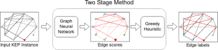
Data availability

The code implemented and the data used in this paper are freely available at https://github.com/pfpimenta/kep_gnn .

Roth A, Sönmez T, Unver U (2004) Kidney exchange. Q J Econ 119(2):457–488

Article   Google Scholar  

Anderson R, Ashlagi I, Gamarnik D, Roth AE (2015) Finding long chains in kidney exchange using the traveling salesman problem. Proc Natl Acad Sci 112(3):663–668. https://doi.org/10.1073/pnas.1421853112

Delorme M, García S, Gondzio J, Kalcsics J, Manlove D, Pettersson W, Trimble J (2022) Improved instance generation for kidney exchange programmes. Comput Oper Res 141:105707. https://doi.org/10.1016/j.cor.2022.105707

Axelrod DA, Schnitzler MA, Xiao H, Irish W, Tuttle-Newhall E, Chang S-H, Kasiske BL, Alhamad T, Lentine KL (2018) An economic assessment of contemporary kidney transplant practice. Am J Transplant 18(5):1168–1176. https://doi.org/10.1111/ajt.14702

Longest Kidney Transplant Chain—Guinness World Record Organization Distinguishes the National Kidney Registry for World’s Longest Kidney Transplant Chain. Accessed: 2023-03-01 (2020). https://transplantsurgery.ucsf.edu/news--events/ucsf-news/88223/UCSF-Part-of-Longest-Kidney-Transplant-Chain---Guinness-World-Record-Organization-Distinguishes-the-National-Kidney-Registry-for-World%E2%80%99s-Longest-Kidney-Transplant-Chain

Biró P, van de Klundert J, Manlove D, Pettersson W, Andersson T, Burnapp L, Chromy P, Delgado P, Dworczak P, Haase B, Hemke A, Johnson R, Klimentova X, Kuypers D, Nanni Costa A, Smeulders B, Spieksma F, Valentín MO, Viana A (2021) Modelling and optimisation in European kidney exchange programmes. Eur J Oper Res 291(2):447–456. https://doi.org/10.1016/j.ejor.2019.09.006

Abraham DJ, Blum A, Sandholm T (2007) Clearing algorithms for barter exchange markets: enabling nationwide kidney exchanges. In: Proceedings of the 8th ACM conference on electronic commerce. EC’07, pp 295–304. Association for Computing Machinery, New York, NY, USA. https://doi.org/10.1145/1250910.1250954

Yang Y, Rajgopal J (2020) Learning combined set covering and traveling salesman problem. arXiv preprint arXiv:2007.03203

Lemos H, Prates MOR, Avelar PHC, Lamb LC (2019) Graph colouring meets deep learning: Effective graph neural network models for combinatorial problems. In: 31st IEEE international conference on tools with artificial intelligence ICTAI, pp 879–885. https://doi.org/10.1109/ICTAI.2019.00125

Santos HLd (2020) Solving the decision version of the graph coloring problem: a neural-symbolic approach using graph neural networks. Master’s thesis, UFRGS Federal University, Porto Alegre, Brazil. https://search.ebscohost.com/login.aspx?direct=true &AuthType=shib &db=cat07377a &AN=sabi.001114939 &lang=pt-br &scope=site &authtype=guest,shib &custid=s5837110 &groupid=main &profile=eds

Sato R, Yamada M, Kashima H (2019) Approximation ratios of graph neural networks for combinatorial problems. In: Wallach HM, Larochelle H, Beygelzimer A, d’Alché-Buc F, Fox EB, Garnett R (eds) Advances in neural information processing systems, vol 32, pp 4083–4092

Abe K, Xu Z, Sato I, Sugiyama M (2019) Solving np-hard problems on graphs with extended AlphaGo zero. arXiv https://doi.org/10.48550/ARXIV.1905.11623

Khalil EB, Dai H, Zhang Y, Dilkina B, Song L (2017) Learning combinatorial optimization algorithms over graphs. In: Guyon I, Luxburg U, Bengio S, Wallach HM, Fergus R, Vishwanathan SVN, Garnett R (eds) Advances in neural information processing systems, vol 30, pp 6348–6358. https://proceedings.neurips.cc/paper/2017/hash/d9896106ca98d3d05b8cbdf4fd8b13a1-Abstract.html

Nazi A, Hang W, Goldie A, Ravi S, Mirhoseini A (2019) Gap: generalizable approximate graph partitioning framework. arXiv https://doi.org/10.48550/ARXIV.1903.00614

Li Z, Chen Q, Koltun V (2018) Combinatorial optimization with graph convolutional networks and guided tree search. In: Bengio S, Wallach HM, Larochelle H, Grauman K, Cesa-Bianchi N, Garnett R (eds) Advances in neural information processing systems, vol 31, pp 537–546. https://proceedings.neurips.cc/paper/2018/hash/8d3bba7425e7c98c50f52ca1b52d3735-Abstract.html

Bai Y, Xu D, Sun Y, Wang W (2021) GLSearch: maximum common subgraph detection via learning to search. In: Meila M, Zhang T (eds) Proceedings of the 38th international conference on machine learning, ICML, pp 588–598. http://proceedings.mlr.press/v139/bai21e.html

Joshi CK, Laurent T, Bresson X (2019) An efficient graph convolutional network technique for the travelling salesman problem. arXiv https://doi.org/10.48550/ARXIV.1906.01227

Joshi CK, Cappart Q, Rousseau L-M, Laurent T (2021) Learning tsp requires rethinking generalization. In: 27th international conference on principles and practice of constraint programming (CP 2021). Schloss Dagstuhl-Leibniz-Zentrum für Informatik

Prates MOR, Avelar PHC, Lemos H, Lamb LC, Vardi MY (2019) Learning to solve np-complete problems: A graph neural network for decision TSP. In: The thirty-third AAAI conference on artificial intelligence, AAAI 2019, pp 4731–4738. https://doi.org/10.1609/aaai.v33i01.33014731

Vinyals O, Fortunato M, Jaitly N (2015) Pointer networks. Adv Neural Inf Process Syst 28:3505

Google Scholar  

Wu Y, Song W, Cao Z, Zhang J, Lim A (2021) Learning improvement heuristics for solving routing problems. IEEE Trans Neural Netw Learn Syst 33(9):5057–5069

Article   MathSciNet   Google Scholar  

Kool W, Hoof H, Welling M (2019) Attention, learn to solve routing problems! In: 7th international conference on learning representations, ICLR 2019, New Orleans, LA, USA, May 6–9, 2019. OpenReview.net. https://openreview.net/forum?id=ByxBFsRqYm

Bello I, Pham H, Le QV, Norouzi M, Bengio S (2017) Neural combinatorial optimization with reinforcement learning. In: 5th international conference on learning representations, ICLR 2017, Toulon, France, April 24–26, 2017, Workshop track proceedings. OpenReview.net. https://openreview.net/forum?id=Bk9mxlSFx

Peng Y, Choi B, Xu J (2021) Graph learning for combinatorial optimization: a survey of state-of-the-art. Data Sci Eng 6(2):119–141. https://doi.org/10.1007/s41019-021-00155-3

Lamb LC, Garcez AS, Gori M, Prates MOR, Avelar PHC, Vardi MY (2020) Graph neural networks meet neural-symbolic computing: a survey and perspective. In: Bessiere C (ed) Proceedings of the twenty-ninth international joint conference on artificial intelligence, IJCAI 2020, pp 4877–4884. https://doi.org/10.24963/ijcai.2020/679

Shervashidze N, Schweitzer P, Leeuwen EJ, Mehlhorn K, Borgwardt KM (2011) Weisfeiler–Lehman graph kernels. J Mach Learn Res 12(77):2539–2561

MathSciNet   Google Scholar  

Lecoutre C, Szczepanski N (2020) PYCSP3: modeling combinatorial constrained problems in python. CoRR arXiv:2009.00326

Roth AE, Sönmez T, Ünver MU (2007) Efficient kidney exchange: coincidence of wants in markets with compatibility-based preferences. Am Econ Rev 97(3):828–851. https://doi.org/10.1257/aer.97.3.828

Constantino M, Klimentova X, Viana A, Rais A (2013) New insights on integer-programming models for the kidney exchange problem. Eur J Oper Res 231(1):57–68. https://doi.org/10.1016/j.ejor.2013.05.025

Corso G, Cavalleri L, Beaini D, Liò P, Velič ković P (2020) Principal neighbourhood aggregation for graph nets. arXiv. https://doi.org/10.48550/ARXIV.2004.05718 . arXiv:2004.05718

Brody S, Alon U, Yahav E (2021) How attentive are graph attention networks? arXiv. https://doi.org/10.48550/ARXIV.2105.14491 . arXiv:2105.14491

Saidman SL, Roth AE, Sönmez T, Ünver MU, Delmonico FL (2006) Increasing the opportunity of live kidney donation by matching for two- and three-way exchanges. Transplantation 81(5):773–782

Simonovsky M, Komodakis N (2018) Graphvae: towards generation of small graphs using variational autoencoders. In: Artificial neural networks and machine learning—ICANN 2018. Lecture Notes in Computer Science, vol 11139, pp 412–422. https://doi.org/10.1007/978-3-030-01418-6_41

De Cao N, Kipf T (2018) Molgan: An implicit generative model for small molecular graphs. arXiv preprint https://doi.org/10.48550/ARXIV.1805.11973 arXiv:1805.11973

Download references

CAPES Finance code (001) and CNPq supported this research in part.

Author information

Authors and affiliations.

Universidade Federal do Rio Grande do Sul, Porto Alegre, Brazil

Pedro F. Pimenta & Luís C. Lamb

King’s College, London, UK

Pedro H. C. Avelar

A*STAR, Singapore, Singapore

You can also search for this author in PubMed   Google Scholar

Corresponding authors

Correspondence to Pedro F. Pimenta or Luís C. Lamb .

Ethics declarations

Conflict of interest.

The authors declare no conflict of interest in this research.

Additional information

Publisher's note.

Springer Nature remains neutral with regard to jurisdictional claims in published maps and institutional affiliations.

Rights and permissions

Springer Nature or its licensor (e.g. a society or other partner) holds exclusive rights to this article under a publishing agreement with the author(s) or other rightsholder(s); author self-archiving of the accepted manuscript version of this article is solely governed by the terms of such publishing agreement and applicable law.

Reprints and permissions

About this article

Pimenta, P.F., Avelar, P.H.C. & Lamb, L.C. Solving the kidney exchange problem via graph neural networks with no supervision. Neural Comput & Applic (2024). https://doi.org/10.1007/s00521-024-09887-5

Download citation

Received : 27 November 2023

Accepted : 23 April 2024

Published : 15 May 2024

DOI : https://doi.org/10.1007/s00521-024-09887-5

Share this article

Anyone you share the following link with will be able to read this content:

Sorry, a shareable link is not currently available for this article.

Provided by the Springer Nature SharedIt content-sharing initiative

• Kidney exchange problem
• Graph neural networks
• Optimization
• Machine learning
• Deep learning
• Graph theory and applications
• Find a journal
• Publish with us
• Track your research

Help | Advanced Search

Mathematics > Optimization and Control

Title: adversarial neural network methods for topology optimization of eigenvalue problems.

Abstract: This research presents a novel method using an adversarial neural network to solve the eigenvalue topology optimization problems. The study focuses on optimizing the first eigenvalues of second-order elliptic and fourth-order biharmonic operators subject to geometry constraints. These models are usually solved with topology optimization algorithms based on sensitivity analysis, in which it is expensive to repeatedly solve the nonlinear constrained eigenvalue problem with traditional numerical methods such as finite elements or finite differences. In contrast, our method leverages automatic differentiation within the deep learning framework. Furthermore, the adversarial neural networks enable different neural networks to train independently, which improves the training efficiency and achieve satisfactory optimization results. Numerical results are presented to verify effectiveness of the algorithms for maximizing and minimizing the first eigenvalues.

Submission history

Access paper:.

• HTML (experimental)
• Other Formats

References & Citations

• Google Scholar
• Semantic Scholar

BibTeX formatted citation

Bibliographic and Citation Tools

Code, data and media associated with this article, recommenders and search tools.

• Institution

arXivLabs: experimental projects with community collaborators

arXivLabs is a framework that allows collaborators to develop and share new arXiv features directly on our website.

Both individuals and organizations that work with arXivLabs have embraced and accepted our values of openness, community, excellence, and user data privacy. arXiv is committed to these values and only works with partners that adhere to them.

Have an idea for a project that will add value for arXiv's community? Learn more about arXivLabs .

• Computer Vision
• Federated Learning
• Reinforcement Learning
• Natural Language Processing
• New Releases
• AI Dev Tools
• Advisory Board Members
• 🐝 Partnership and Promotion

Shobha Kakkar

Shobha is a data analyst with a proven track record of developing innovative machine-learning solutions that drive business value.

• 30+ AI Tools For Startups in 2024
• Top 50 AI Writing Tools To Try in 2024
• Top Machine Learning Courses for Finance
• Top Low/No Code AI Tools 2024

RELATED ARTICLES MORE FROM AUTHOR

Top ai tools for real estate agents, phidata: an ai framework for building autonomous assistants with long-term memory, contextual knowledge and the ability to take actions using function calling, numind releases three sota ner models that outperform similar-sized foundation models in the few-shot regime and competing with much larger llms, agentclinic: simulating clinical environments for assessing language models in healthcare, consistency large language models (cllms): a new family of llms specialized for the jacobi decoding method for latency reduction, this ai paper by toyota research institute introduces supra: enhancing transformer efficiency with recurrent neural networks, numind releases three sota ner models that outperform similar-sized foundation models in the few-shot..., phidata: an ai framework for building autonomous assistants with long-term memory, contextual knowledge and the..., consistency large language models (cllms): a new family of llms specialized for the jacobi....

• AI Magazine
• Privacy & TC
• Cookie Policy

🐝 🐝 Join the Fastest Growing AI Research Newsletter Read by Researchers from Google + NVIDIA + Meta + Stanford + MIT + Microsoft and many others...

Thank You 🙌

Privacy Overview