correlation hypothesis test python

Statistics Made Easy

How to Perform a Correlation Test in Python (With Example)

One way to quantify the relationship between two variables is to use the Pearson correlation coefficient , which measures the linear association between two variables .

It always takes on a value between -1 and 1 where:

• -1 indicates a perfectly negative linear correlation
• 0 indicates no linear correlation
• 1 indicates a perfectly positive linear correlation

To determine if a correlation coefficient is statistically significant, you can calculate the corresponding t-score and p-value.

The formula to calculate the t-score of a correlation coefficient (r) is:

t = r * √ n-2 / √ 1-r 2

The p-value is then calculated as the corresponding two-sided p-value for the t-distribution with n-2 degrees of freedom.

Example: Correlation Test in Python

To determine if the correlation coefficient between two variables is statistically significant, you can perform a correlation test in Python using the pearsonr function from the SciPy library.

This function returns the correlation coefficient between two variables along with the two-tailed p-value.

For example, suppose we have the following two arrays in Python:

We can import the pearsonr function and calculate the Pearson correlation coefficient between the two arrays:

Here’s how to interpret the output:

• Pearson correlation coefficient (r): 0.8076
• Two-tailed p-value: 0.0047

Since the correlation coefficient is close to 1, this tells us that there is a strong positive association between the two variables.

And since the corresponding p-value is less than .05, we conclude that there is a statistically significant association between the two variables.

Note that we can also extract the individual correlation coefficient and p-value from the pearsonr function as well:

These values are a bit easier to read compared to the output from the original pearsonr function.

Additional Resources

The following tutorials provide additional information about correlation coefficients:

An Introduction to the Pearson Correlation Coefficient What is Considered to Be a “Strong” Correlation? The Five Assumptions for Pearson Correlation

Featured Posts

Hey there. My name is Zach Bobbitt. I have a Masters of Science degree in Applied Statistics and I’ve worked on machine learning algorithms for professional businesses in both healthcare and retail. I’m passionate about statistics, machine learning, and data visualization and I created Statology to be a resource for both students and teachers alike.  My goal with this site is to help you learn statistics through using simple terms, plenty of real-world examples, and helpful illustrations.

Leave a Reply Cancel reply

Your email address will not be published. Required fields are marked *

Join the Statology Community

Sign up to receive Statology's exclusive study resource: 100 practice problems with step-by-step solutions. Plus, get our latest insights, tutorials, and data analysis tips straight to your inbox!

By subscribing you accept Statology's Privacy Policy.

Statistical Hypothesis Analysis in Python with ANOVAs, Chi-Square, and Pearson Correlation

• Introduction

Python is an incredibly versatile language, useful for a wide variety of tasks in a wide range of disciplines. One such discipline is statistical analysis on datasets, and along with SPSS, Python is one of the most common tools for statistics.

Python's user-friendly and intuitive nature makes running statistical tests and implementing analytical techniques easy, especially through the use of the statsmodels library .

• Introducing the statsmodels Library in Python

The statsmodels library is a module for Python that gives easy access to a variety of statistical tools for carrying out statistical tests and exploring data. There are a number of statistical tests and functions that the library grants access to, including ordinary least squares (OLS) regressions, generalized linear models, logit models, Principal Component Analysis (PCA) , and Autoregressive Integrated Moving Average (ARIMA) models.

The results of the models are constantly tested against other statistical packages to ensure that the models are accurate. When combined with SciPy and Pandas , it's simple to visualize data, run statistical tests, and check relationships for significance.

• Choosing a Dataset

Before we can practice statistics with Python, we need to select a dataset. We'll be making use of a dataset compiled by the Gapminder Foundation.

The Gapminder Dataset tracks many variables used to assess the general health and wellness of populations in countries around the world. We'll be using the dataset because it is very well documented, standardized, and complete. We won't have to do much in the way of preprocessing in order to make use of it.

There are a few things we'll want to do just to get the dataset ready to run regressions, ANOVAs, and other tests, but by and large the dataset is ready to work with.

The starting point for our statistical analysis of the Gapminder dataset is exploratory data analysis. We'll use some graphing and plotting functions from Matplotlib and Seaborn to visualize some interesting relationships and get an idea of what variable relationships we may want to explore.

• Exploratory Data Analysis and Preprocessing

We'll start off by visualizing some possible relationships. Using Seaborn and Pandas we can do some regressions that look at the strength of correlations between the variables in our dataset to get an idea of which variable relationships are worth studying.

We'll import those two and any other libraries we'll be using here:

There isn't much preprocessing we have to do, but we do need to do a few things. First, we'll check for any missing or null data and convert any non-numeric entries to numeric. We'll also make a copy of the transformed dataframe that we'll work with:

Here are the outputs:

There's a handful of missing values, but our numeric conversion should turn them into NaN values, allowing exploratory data analysis to be carried out on the dataset.

Specifically, we could try analyzing the relationship between internet use rate and life expectancy, or between internet use rate and employment rate. Let's try making individual graphs of some of these relationships using Seaborn and Matplotlib:

Here are the results of the graphs:

It looks like there are some interesting relationships that we could further investigate. Interestingly, there seems to be a fairly strong positive relationship between internet use rate and breast cancer, though this is likely just an artifact of better testing in countries that have more access to technology.

There also seems to be a fairly strong, though less linear relationship between life expectancy and internet use rate.

Finally, it looks like there is a parabolic, non-linear relationship between internet use rate and employment rate.

• Selecting a Suitable Hypothesis

We want to pick out a relationship that merits further exploration. There are many potential relationships here that we could form a hypothesis about and explore the relationship with statistical tests. When we make a hypothesis and run a correlation test between the two variables, if the correlation test is significant, we then need to conduct statistical tests to see just how strong the correlation is and if we can reliably say that the correlation between the two variables is more than just chance.

The type of statistical test we use will depend on the nature of our explanatory and response variables, also known and independent and dependent variables . We'll go over how to run three different types of statistical tests:

• Chi-Square Tests
• Regressions.

We'll go with what we visualized above and choose to explore the relationship between internet use rates and life expectancy.

The null hypothesis is that there is no significant relationship between internet use rate and life expectancy, while our hypothesis is that there is a relationship between the two variables.

We're going to be conducting various types of hypothesis tests on the dataset. The type of hypothesis test that we use is dependent on the nature of our explanatory and response variables. Different combinations of explanatory and response variables require different statistical tests. For example, if one variable is categorical and one variable is quantitative in nature, an Analysis of Variance is required.

• Analysis of Variance (ANOVA)

An Analysis of Variance (ANOVA) is a statistical test employed to compare two or more means together, which are determined through the analysis of variance. One-way ANOVA tests are utilized to analyze differences between groups and determine if the differences are statistically significant.

One-way ANOVAs compare two or more independent group means, though in practice they are most often used when there are at least three independent groups.

In order to carry out an ANOVA on the Gapminder dataset, we'll need to transform some of the features, as these values in the dataset are continuous but ANOVA analyses are appropriate for situations where one variable is categorical and one variable is quantitative.

We can transform the data from continuous to quantitative by selecting a category and binning the variable in question, dividing it into percentiles. The independent variable will be converted into a categorical variable, while the dependent variable will stay continuous. We can use the qcut() function in Pandas to divide the dataframe into bins:

After the variables have been transformed and are ready to be analyzed, we can use the statsmodel library to carry out an ANOVA on the selected features. We'll print out the results of the ANOVA and check to see if the relationship between the two variables is statistically significant:

Here's the output of the model:

We can see that the model gives a very small P-value ( Prob F-statistic ) of 1.71e-35 . This is far less than the usual significance threshold of 0.05 , so we conclude there is a significant relationship between life expectancy and internet use rate.

Since the correlation P-value does seem to be significant, and since we have 10 different categories, we'll want to run a post-hoc test to check that the difference between the means is still significant even after we check for type-1 errors. We can carry out post-hoc tests with the help of the multicomp module, utilizing a Tukey Honestly Significant Difference (Tukey HSD) test:

Here are the results of the test:

Now we have some better insight into which groups in our comparison have statistically significant differences.

If the reject column has a label of False , we know it's recommended that we reject the null hypothesis and assume that there is a significant difference between the two groups being compared.

• The Chi-Square Test of Independence

ANOVA is appropriate for instances where one variable is continuous and the other is categorical. Now we'll be looking at how to carry out a Chi-Square test of independence .

The Chi-Square test of independence is utilized when both explanatory and response variables are categorical. You likely also want to use the Chi-Square test when the explanatory variable is quantitative and the response variable is categorical, which you can do by dividing the explanatory variable into categories.

Check out our hands-on, practical guide to learning Git, with best-practices, industry-accepted standards, and included cheat sheet. Stop Googling Git commands and actually learn it!

The Chi-Square test of independence is a statistical test used to analyze how significant a relationship between two categorical variables is. When a Chi-Square test is run, every category in one variable has its frequency compared against the second variable's categories. This means that the data can be displayed as a frequency table, where the rows represent the independent variables and the columns represent the dependent variables.

Much like we converted our independent variable into a categorical variable (by binning it), for the ANOVA test, we need to make both variables categorical in order to carry out the Chi-Square test. Our hypothesis for this problem is the same as the hypothesis in the previous problem, that there is a significant relationship between life expectancy and internet use rate.

We'll keep things simple for now and divide our internet use rate variable into two categories, though we could easily do more. We'll write a function to handle that.

We'll be conducting post-hoc comparison to guard against type-1 errors (false positives) using an approach called the Bonferroni Adjustment . In order to do this, you can carry out comparisons for the different possible pairs of your response variable, and then you check their adjusted significance.

We won't run comparisons for all the different possible pairs here, we'll just show how it can be done. We'll make a few different comparisons using a re-coding scheme and map the records into new feature columns.

Afterwards, we can check the observed counts and create tables of those comparisons:

Running a Chi-Square test and post-hoc comparison involves first constructing a cross-tabs comparison table. The cross-tabs comparison table shows the percentage of occurrence for the response variable for the different levels of the explanatory variable.

Just to get an idea of how this works, let's print out the results for all the life expectancy bin comparisons:

We can see that a cross-tab comparison checks for the frequency of one variable's categories in the second variable. Above we see the distribution of life expectancies in situations where they fall into one of the two bins we created.

Now we need to compute the cross-tabs for the different pairs we created above, as this is what we run through the Chi-Square test:

Once we have transformed the variables so that the Chi-Square test can be carried out, we can use the chi2_contingency function in statsmodel to carry out the test.

We want to print out the column percentages as well as the results of the Chi-Square test, and we'll create a function to do this. We'll then use our function to do the Chi-Square test for the four comparison tables we created:

Here are the results:

If we're only looking at the results for the full count table, it looks like there's a P-value of 6.064860600653971e-18 .

However, in order to ascertain how the different groups diverge from one another, we need to carry out the Chi-Square test for the different pairs in our dataframe. We'll check to see if there is a statistically significant difference for each of the different pairs we selected. Note that the P-value which indicates a significant result changes depending on how many comparisons you are making, and while we won't cover that in this tutorial, you'll need to be mindful of it.

The 6 vs 9 comparison gives us a P-value of 0.127 , which is above the 0.05 threshold, indicating that the difference for that category may be non-significant. Seeing the differences of the comparisons helps us understand why we need to compare different levels with one another.

• Pearson Correlation

We've covered the test you should use when you have a categorical explanatory variable and a quantitative response variable (ANOVA), as well as the test you use when you have two categorical variables (Chi-Squared).

We'll now take a look at the appropriate type of test to use when you have a quantitative explanatory variable and a quantitative response variable - the Pearson Correlation .

The Pearson Correlation test is used to analyze the strength of a relationship between two provided variables, both quantitative in nature. The value, or strength of the Pearson correlation, will be between +1 and -1 .

A correlation of 1 indicates a perfect association between the variables, and the correlation is either positive or negative. Correlation coefficients near 0 indicate very weak, almost non-existent, correlations. While there are other ways of measuring correlations between two variables, such as Spearman Correlation or Kendall Rank Correlation , the Pearson correlation is probably the most commonly used correlation test.

As the Gapminder dataset has its features represented with quantitative variables, we don't need to do any categorical transformation of the data before running a Pearson Correlation on it. Note that it's assumed that both variables are normally distributed and there aren't many significant outliers in the dataset. We'll need access to SciPy in order to carry out the Pearson correlation.

We'll graph the relationship between life expectancy and internet use rates, as well as internet use rate and employment rate, just to see what another correlation graph might look like. After creating a graphing function, we'll use the pearsonr() function from SciPy to carry out the correlation and check the results:

The first value is the direction and strength of the correlation, while the second is the P-value. The numbers suggest a fairly strong correlation between life expectancy and internet use rate that isn't due to chance. Meanwhile, there's a weaker, though still significant correlation between employment rate and internet use rate.

Note that it is also possible to run a Pearson Correlation on categorical data, though the results will look somewhat different. If we wanted to, we could group the income levels and run the Pearson Correlation on them. You can use it to check for the presence of moderating variables that could be having an effect on your association of interest.

• Moderators and Statistical Interaction

Let's look at how to account for statistical interaction between multiple variables, AKA moderation.

Moderation is when a third (or more) variable impacts the strength of the association between the independent variable and the dependent variable.

There are different ways to test for moderation/statistical interaction between a third variable and the independent/dependent variables. For example, if you carried out an ANOVA test, you could test for moderation by doing a two-way ANOVA test in order to test for possible moderation.

However, a reliable way to test for moderation, no matter what type of statistical test you ran (ANOVA, Chi-Square, Pearson Correlation) is to check if there is an association between explanatory and response variables for every subgroup/level of the third variable.

To be more concrete, if you were carrying out ANOVA tests, you could just run an ANOVA for every category in the third variable (the variable you suspect might have a moderating effect on the relationship you are studying).

If you were using a Chi-Square test, you could just carry out a Chi-Square test on new dataframes holding all data points found within the categories of your moderating variable.

If your statistical test is a Pearson correlation, you would need to create categories or bins for the moderating variable and then run the Pearson correlation for all three of those bins.

Let's take a quick look at how to carry out Pearson Correlations for moderating variables. We'll create artificial categories/levels out of our continuous features. The process for testing for moderation for the other two test types (Chi-Square and ANOVA) is very similar, but you'll have pre-existing categorical variables to work with instead.

We'll want to choose a suitable variable to act as our moderating variable. Let's try income level per person and divide it into three different groups:

Once more, the first value is the direction and strength of the correlation, while the second is the P-value.

statsmodels is an extremely useful library that allows Python users to analyze data and run statistical tests on datasets. You can carry out ANOVAs, Chi-Square Tests, Pearson Correlations and tests for moderation.

Once you become familiar with how to carry out these tests, you'll be able to test for significant relationships between dependent and independent variables, adapting for the categorical or continuous nature of the variables.

You might also like...

• Keras Callbacks: Save and Visualize Prediction on Each Training Epoch
• Loading a Pretrained TensorFlow Model into TensorFlow Serving
• Scikit-Learn's train_test_split() - Training, Testing and Validation Sets
• Feature Scaling Data with Scikit-Learn for Machine Learning in Python

Improve your dev skills!

Get tutorials, guides, and dev jobs in your inbox.

No spam ever. Unsubscribe at any time. Read our Privacy Policy.

Aspiring data scientist and writer. BS in Communications. I hope to use my multiple talents and skillsets to teach others about the transformative power of computer programming and data science.

In this article

Bank Note Fraud Detection with SVMs in Python with Scikit-Learn

Can you tell the difference between a real and a fraud bank note? Probably! Can you do it for 1000 bank notes? Probably! But it...

Building Your First Convolutional Neural Network With Keras

Most resources start with pristine datasets, start at importing and finish at validation. There's much more to know. Why was a class predicted? Where was...

© 2013- 2024 Stack Abuse. All rights reserved.

Nick McCullum

Software Developer & Professional Explainer

A Guide to Python Correlation Statistics with NumPy, SciPy, & Pandas

When dealing with data, it's important to establish the unknown relationships between various variables.

Other than discovering the relationships between the variables, it is important to quantify the degree to which they depend on each other.

Such statistics can be used in science and technology.

Python provides its users with tools that they can use to calculate these statistics.

In this article, I will help you know how to use SciPy, Numpy, and Pandas libraries in Python to calculate correlation coefficients between variables.

Table of Contents

You can skip to a specific section of this Python correlation statistics tutorial using the table of contents below:

What is Correlation?

Correlation calculation using numpy, correlation calculation using scipy, correlation calculation in pandas, linear correlation, pearson correlation coefficient, linear regression in scipy, pearson correlation in numpy and scipy, pearson correlation in pandas, rank correlation, spearman correlation coefficient, kendall correlation coefficient, scipy implementation of rank, rank correlation implementation in numpy and scipy, rank correlation implementation in pandas, visualizing correlation, heatmaps of correlation matrices, final thoughts.

The variables within a dataset may be related in different ways.

For example,

One variable may be dependent on the values of another variable, two variables may be dependent on a third unknown variable, etc.

It will be better in statistics and data science to determine the undelying relationship between variables.

Correlation is the measure of how two variables are strongly related to each other.

Once data is organized in the form of a table, the rows of the table become the observations while the columns become the features or the attributes .

There are three types of correlation.

They include:

Negative correlation- This is a type of correlation in which large values of one feature correspond to small values of another feature.

If you plot this relationship on a cartesian plane, the y values will decrease as the x values increase.

The vice versa is also true, that small values of one feature correspond to large features of another feature.

If you plot this relationship on a cartesian plane, the y values will increase as the x values decrease.

Weak or no correlation- In this type of correlation, there is no observable association between two features.

The reason is that the correlation between the two variables is weak.

Positive correlation- In this type of correlation, large values for one feature correspond to large values for another feature.

When plotted, the values of y tend to increase with an increase in the values of x, showing a strong correlation between the two.

Correlation goes hand-in-hand with other statistical quantities like the mean, variance, standard deviation, and covariance.

In this article, we will be focussing on the three major correlation coefficients.

These include:

• Pearson’s r
• Spearman’s rho
• Kendall’s tau

The Pearson's coefficient helps to measure linear correlation, while the Kendal and Spearman coeffients helps compare the ranks of data.

The SciPy, NumPy, and Pandas libraries come with numerous correlation functions that you can use to calculate these coefficients.

If you need to visualize the results, you can use Matplotlib .

NumPy comes with many statistics functions.

An example is the np.corrcoef() function that gives a matrix of Pearson correlation coefficients.

To use the NumPy library, we should first import it as shown below:

Next, we can use the ndarray class of NumPy to define two arrays.

We will call them x and y :

You can see the generated arrays by typing their names on the Python terminal as shown below:

First, we have used the np.arange() function to generate an array given the name x with values ranging between 10 and 20, with 10 inclusive and 20 exclusive.

We have then used np.array() function to create an array of arbitrary integers.

We now have two arrays of equal length.

You can use Matplotlib to plot the datapoints:

This will return the following plot:

The colored dots are the datapoints.

It's now time for us to determine the relationship between the two arrays.

We will simply call the np.corrcoef() function and pass to it the two arrays as the arguments.

This is shown below:

Now, type corr on the Python terminal to see the generated correlation matrix:

The correlation matrix is a two-dimensional array showing the correlation coefficients.

If you've observed keenly, you must have noticed that the values on the main diagonal, that is, upper left and lower right, equal to 1.

The value on the upper left is the correlation coefficient for x and x .

The value on the lower right is the correlation coefficient for y and y .

In this case, it's approximately 8.2.

They will always give a value of 1.

However, the lower left and the upper right values are of the most signicance and you will need them frequently.

The two values are equal and they denote the pearson correlation coefficient for variables x and y .

SciPy has a module called scipy.stats that comes with many routines for statistics.

To calculate the three coefficients that we mentioned earlier, you can call the following functions:

• spearmanr()
• kendalltau()

Let me show you how to do it...

First, we import numpy and the scipy.stats module from SciPy.

Next, we can generate two arrays.

You can calculate the Pearson's r coefficient as follows:

This should return the following:

The value for Spearman's rho can be calculated as follows:

You should get this:

And finally, you can calculate the Kendall's tau as follows:

The output should be as follows:

The output from each of the three functions has two values.

The first value is the correlation coefficient while the second value is the p-value.

In this case, our great focus is on the coefficient correlation, the first value.

The p-value becomes useful when testing hypothesis in statistical methods.

If you only want to get the correlation coefficient, you can extract it using its index.

Since it's the first value, it's located at index 0.

The following demonstrates this:

Each should return one value as shown below:

In some cases, the Pandas library is more convenient for calculating statistics compared to NumPy and SciPy.

It comes with statistical methods for DataFrame and Series data instances.

For example, if you have two Series objects with equal number of items, you can call the .corr() function on one of them with the other as the first argument.

First, let's import the Pandas library and generate a Series data object with a set of integers:

To see the generated Series, type x on Python terminal:

It has generated numbers between 20 and 30, with 20 inclusive and 30 exclusive.

We can generate the second Series object:

To see the values for this series object, type y on the Python terminal:

To calculate the Pearson's r coefficient for x in relation to y , we can call the .corr() function as follows:

This returns the following:

The Pearson's r coefficient for y in relation to x can be calculated as follows:

You can then calculate the Spearman's rho as follows:

Note that we had to set the parameter method to spearman .

It should return the following:

The Kendall's tau can then be calculated as follows:

It returns the following:

The method parameter was set to kendall .

The purpose of linear correlation is to measure the proximity of a mathematical relationship between the variables of a dataset to a linear function.

If the relationship between the two variables is found to be closer to a linear function, then they have a stronger linear correlation and the absolute value of the correlation coefficient is higher.

Let's say you have a dataset with two features, x and y .

Each of these features has n values, meaning that x and y are n tuples.

The first value of feature x , x1 corresponds to the first value of feature y , y1 .

The second value of feature x , x2 , corresponds to the second value of feature y , y2 .

Each of the x-y pairs denotes a single observation.

The Pearson (product-moment) correlation coefficient measures the linear relationship between two features.

It is simply the ratio of the covariance of x and y to the product of their standard deviations.

It is normally denoted using the letter r and it can be expressed using the following mathematical equation:

r = Σᵢ((xᵢ − mean(x))(yᵢ − mean(y))) (√Σᵢ(xᵢ − mean(x))² √Σᵢ(yᵢ − mean(y))²)⁻¹

The parameter i can take the values 1, 2,...n.

The mean values for x an y can be denoted as mean(x) and mean(y) respectively.

Note the following facts regarding the Pearson correlation coefficient:

• It can take any real values ranging between −1 ≤ r ≤ 1.
• The maximum value of r is 1, and it denotes a case where there exists a perfect positive linear relationship between x and y .
• If r > 0, there is a positive correlation between x and y .
• If r = 0, x and y are independent.
• If r < 0, there is a negative correlation between x and y .
• The minimum value of r is 1, and it denotes a case where there is a perfect negative linear relationship between x and y .

So, a larger absolute value of r is an indication of a stronger correlation, closer to a linear function.

While, a smaller absolute value of r is an indication of a weaker correlation.

SciPy can give us a linear function that best approximates the existing relationship between two arrays and the Pearson correlation coefficient.

So, let's first import the libraries and prepare the data:

Now that the data is ready, we can call the scipy.stats.linregress() function and perform linear regression.

We are performing linear regression between the two features, x and y .

Let's get the values of different coefficients:

These should run as follows:

So, you've used linear regression to get the following values:

• slope- This is the slope for the regression line.
• intercept- This is the intercept for the regression line.
• pvalue- This is the p-value.
• stderr- This is the standard error for the estimated gradient.

At this point, you know how to use the corrcoef() and pearsonr() functions to calculate the Pearson correlation coefficient.

Run the above command then access the values of r and p by typing them on the terminal.

The value of r should be as follows:

The value of p should be as follows:

Here is how to use the corrcoef() function:

Note that if you pass an array with a nan value to the pearsonr() function, it will return a ValueError .

There are a number of details that you should consider.

First, remember that the np.corrcoef() function can take two NumPy arrays as arguments.

You can instead pass to it a two-dimensional array with similar values as the argument.

Let's first create the two-dimensional array:

Let's now call the function:

We get similar results as in the previous examples.

So, let's see what happens when you pass nan data to corrcoef() :

In the above example, the third row of the array has a nan value.

Every calculation that didn't involve the feature with nan value was calculated well.

However, all the results that dependent on the last row are nan .

First, let's import the Pandas library and create Series and DataFrame data objects:

Above, we have created two Series data obects named x , y , and z and two DataFrame data objects named xy and xyz .

To see any of them, type its name on the Python terminal.

See the use of the sys library.

It has helped us provide output information to the Python interpreter.

At this point, you know how to use the .corr() function on Series data objects to get the correlation coefficients.

The above returns the following:

We called the .corr() function on one object and passed the other object to the function as an argument.

The .corr() function can also be used on DataFrame objects.

It can give you the correlation matrix for the columns of the DataFrame object:

For example:

The above code gives us the correlation matrix for the columns of the xy DataFrame object.

To see the generated correlation matrix, type its name on the Python terminal:

The resulting correlation matrix is a new instance of DataFrame and it has the correlation coefficients for the columns xy['x-values'] and xy['y-values'] .

Such labeled results are very convenient to work with since they can be accessed with either their labels or with their integer position indices.

The two run as follows:

The above examples show that there are two ways for you to access the values:

• The .at[] accesses a single value by row and column labels.
• The .iat[] accesses a value based on its row and column positions.

Rank correlation compares the orderings or the ranks of the data related to two features or variables of a dataset.

If the orderings are found to be similar, then the correlation is said to be strong, positive, and high.

On the other hand, if the orderings are found to be close to reversed, the correlation is said to be strong, negative, and low.

This is the Pearson correlation coefficient between the rank values of two features.

It's calculated just as the Pearson correlation coefficient but it uses the ranks instead of their values.

It's denoted using the Greek letter rho (ρ), the Spearman’s rho.

Here are important points to note concerning the Spearman correlation coefficient:

• The ρ can take a value in the range of −1 ≤ ρ ≤ 1.
• The maximum value of ρ is 1, and it corresponds to a case where there is a monotonically increasing function between x and y. Larger values of x correspond to larger values of y. The vice versa is also true.
• The minimum value of ρ is -1, and it corresponds to a case where there is a monotonically decreasing function between x and y. Larger values of x correspond to smaller values of y. The vice versa is also true.

Let's consider two n-tuples again, x and y .

Each x-y , pair, (x1, y1) ..., denotes a single observation.

Each pair of observations, (xᵢ, yᵢ) , and (xⱼ, yⱼ) , where i < j , will be one of the following:

• concordant if (xᵢ > xⱼ and yᵢ > yⱼ) or (xᵢ < xⱼ and yᵢ < yⱼ)
• discordant if (xᵢ < xⱼ and yᵢ > yⱼ) or (xᵢ > xⱼ and yᵢ < yⱼ)
• neither if a tie exists in either x (xᵢ = xⱼ) or in y (yᵢ = yⱼ)

The Kendall correlation coefficient helps us compare the number of concordant and discordant data pairs.

The coefficient shows the difference in the counts of concordant and discordant pairs in relation to the number of x-y pairs.

Note the following points concerning the Kendall correlation coefficient:

• It takes a real value in the range of −1 ≤ τ ≤ 1.
• It has a maximum value of τ = 1 which corresponds to a case when all pairs are concordant.
• It has a minimum value of τ = −1 which corresponds to a case when all pairs are discordant.

The scipy.stats can help you determine the rank of each value in an array.

Let's first import the libraries and create NumPy arrays:

Now that the data is ready, let's use the scipy.stats.rankdata() to calculate the rank of each value in a NumPy array:

The commands return the following:

The array x is monotonic, hence, its rank is also monotonic.

The rankdata() function also takes the optional parameter method .

This tells the Python compiler what to do in case of ties in the array.

By default, the parameter will assign them the average of the ranks.

In the above array, there are two values with a value of 2.

Their total rank is 3.

When averaged, each value got a rank of 1.5.

You can also get ranks using the np.argsort() function.

Which returns the following ranks:

The argsort() function returns the indices of the array items in the asorted array.

The indices are zero-based, so, you have to add 1 to all of them.

You can use the scipy.stats.spearmanr() to calculate the Spearman correlation coefficient.

This runs as follows:

The values for both the correlation coefficient and the pvalue have been shown.

The rho value can be calculated as follows:

This will run as follows:

So, the spearmanr() function returns an object with the value of Spearman correlation coefficient and p-value.

To get the Kendall correlation coefficient, you can use the kendalltau() function as shown below:

The commands will run as follows:

You can use the Pandas library to calculate the Spearman and kendall correlation coefficients.

First, import the Pandas library and create the Series and DataFrame data objects:

You can now call the .corr() and .corrwith() functions and use the method parameter to specify the correlation coefficient that you want to calculate.

It defaults to pearson .

Consider the code given below:

That's how to use the method parameter with the .corr() function.

To calculate the Kendall's tau, use method=kendall .

The commands will return the following output:

Visualizing your data can help you gain more insights about the data.

Luckily, you can use Matplotlib to visualize your data in Python.

If you haven't installed the library, install it using the pip package manager.

Just run the following command:

Next, import its pyplot module by running the following command:

You can then create the arrays of data that you will use to generate the plot:

The data is now ready, hence, you can draw the plot.

We will first demonstrate how to create an x-y plot with a regression line, equation, and Pearson correlation coefficient.

You can use the linregress() function to get the slope, the intercept, and the correlation coefficient for the line.

First, import the stats module from SciPy:

Then run this code:

Also, you can get the string with the equation of regression line and the value of correlation coefficient.

You can use f-strings:

Note that the above line will only work if you are using Python 3.6 and above (f-strings were introduced in Python 3.6).

Now, let's call the .plot() function to generate the x-y plot:

The code will generate the following plot:

The blue squares on the plot denote the observations, while the yellow line is the regression line.

The correlation matrix can be big and confusing when you are handling a huge number of features.

However, you can use a heat map to present it and each field will have a color that corresponds to its value.

You should have a correlation matrix, so, let's create it.

First, this is our array:

Now, let's generate the correlation matrix:

When you type the name of the correlation matrix on the Python terminal, you will get this:

You can now use the .imshow() function to create the heatmap, and pass the name of the correlation matrix to it as the argument:

The following heatmap will be generated:

The result shows a table with coefficients.

The colors on the heatmap will help you interpret the output.

We have three different colors representing different numbers.

This is what you've learned in this article:

• Correlation coeffients measure the association between the features or variables of a dataset.
• The most popular correlation coefficients include the Pearson’s product-moment correlation coefficient, Spearman’s rank correlation coefficient, and Kendall’s rank correlation coefficient.
• The NumPy, Pandas, and SciPy libraries come with functions that you can use to calculate the values of these correlation coefficients.
• Visualing your data will help you gain more insights from the data.
• You can use Matplotlib to visualize your data in Python.

Visual Design.

Upgrade to get unlimited access ($10 one off payment).

7 Tips for Beginner to Future-Proof your Machine Learning Project

LLM Prompt Engineering Techniques for Knowledge Graph Integration

Develop a Data Analytics Web App in 3 Steps

What Does ChatGPT Say About Machine Learning Trend and How Can We Prepare For It?

• Apr 14, 2022

An Interactive Guide to Hypothesis Testing in Python

Updated: Jun 12, 2022

upgrade and grab the cheatsheet from our infographics gallery

What is hypothesis testing.

Hypothesis testing is an essential part in inferential statistics where we use observed data in a sample to draw conclusions about unobserved data - often the population.

Implication of hypothesis testing:

clinical research: widely used in psychology, biology and healthcare research to examine the effectiveness of clinical trials

A/B testing: can be applied in business context to improve conversions through testing different versions of campaign incentives, website designs ...

feature selection in machine learning: filter-based feature selection methods use different statistical tests to determine the feature importance

college or university: well, if you major in statistics or data science, it is likely to appear in your exams

For a brief video walkthrough along with the blog, check out my YouTube channel.

4 Steps in Hypothesis testing

Step 1. define null and alternative hypothesis.

Null hypothesis (H0) can be stated differently depends on the statistical tests, but generalize to the claim that no difference, no relationship or no dependency exists between two or more variables.

Alternative hypothesis (H1) is contradictory to the null hypothesis and it claims that relationships exist. It is the hypothesis that we would like to prove right. However, a more conservational approach is favored in statistics where we always assume null hypothesis is true and try to find evidence to reject the null hypothesis.

Step 2. Choose the appropriate test

Common Types of Statistical Testing including t-tests, z-tests, anova test and chi-square test

T-test: compare two groups/categories of numeric variables with small sample size

Z-test: compare two groups/categories of numeric variables with large sample size

ANOVA test: compare the difference between two or more groups/categories of numeric variables

Chi-Squared test: examine the relationship between two categorical variables

Correlation test: examine the relationship between two numeric variables

Step 3. Calculate the p-value

How p value is calculated primarily depends on the statistical testing selected. Firstly, based on the mean and standard deviation of the observed sample data, we are able to derive the test statistics value (e.g. t-statistics, f-statistics). Then calculate the probability of getting this test statistics given the distribution of the null hypothesis, we will find out the p-value. We will use some examples to demonstrate this in more detail.

Step 4. Determine the statistical significance

p value is then compared against the significance level (also noted as alpha value) to determine whether there is sufficient evidence to reject the null hypothesis. The significance level is a predetermined probability threshold - commonly 0.05. If p value is larger than the threshold, it means that the value is likely to occur in the distribution when the null hypothesis is true. On the other hand, if lower than significance level, it means it is very unlikely to occur in the null hypothesis distribution - hence reject the null hypothesis.

Hypothesis Testing with Examples

Kaggle dataset “ Customer Personality Analysis” is used in this case study to demonstrate different types of statistical test. T-test, ANOVA and Chi-Square test are sensitive to large sample size, and almost certainly will generate very small p-value when sample size is large . Therefore, I took a random sample (size of 100) from the original data:

T-test is used when we want to test the relationship between a numeric variable and a categorical variable.There are three main types of t-test.

one sample t-test: test the mean of one group against a constant value

two sample t-test: test the difference of means between two groups

paired sample t-test: test the difference of means between two measurements of the same subject

For example, if I would like to test whether “Recency” (the number of days since customer’s last purchase - numeric value) contributes to the prediction of “Response” (whether the customer accepted the offer in the last campaign - categorical value), I can use a two sample t-test.

The first sample would be the “Recency” of customers who accepted the offer:

The second sample would be the “Recency” of customers who rejected the offer:

To compare the “Recency” of these two groups intuitively, we can use histogram (or distplot) to show the distributions.

It appears that positive response have lower Recency compared to negative response. To quantify the difference and make it more scientific, let’s follow the steps in hypothesis testing and carry out a t-test.

Step1. define null and alternative hypothesis

null: there is no difference in Recency between the customers who accepted the offer in the last campaign and who did not accept the offer

alternative: customers who accepted the offer has lower Recency compared to customers who did not accept the offer

Step 2. choose the appropriate test

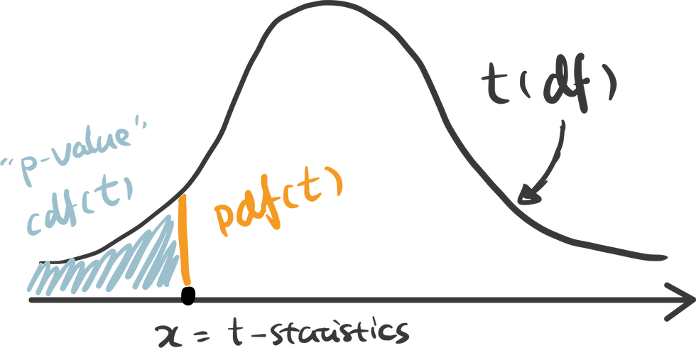
To test the difference between two independent samples, two-sample t-test is the most appropriate statistical test which follows student t-distribution. The shape of student-t distribution is determined by the degree of freedom, calculated as the sum of two sample size minus 2.

In python, simply import the library scipy.stats and create the t-distribution as below.

Step 3. calculate the p-value

There are some handy functions in Python calculate the probability in a distribution. For any x covered in the range of the distribution, pdf(x) is the probability density function of x — which can be represented as the orange line below, and cdf(x) is the cumulative density function of x — which can be seen as the cumulative area. In this example, we are testing the alternative hypothesis that — Recency of positive response minus the Recency of negative response is less than 0. Therefore we should use a one-tail test and compare the t-statistics we get against the lowest value in this distribution — therefore p-value can be calculated as cdf(t_statistics) in this case.

ttest_ind() is a handy function for independent t-test in python that has done all of these for us automatically. Pass two samples rececency_P and recency_N as the parameters, and we get the t-statistics and p-value.

Here I use plotly to visualize the p-value in t-distribution. Hover over the line and see how point probability and p-value changes as the x shifts. The area with filled color highlights the p-value we get for this specific test.

Check out the code in our Code Snippet section, if you want to build this yourself.

An interactive visualization of t-distribution with t-statistics vs. significance level.

Step 4. determine the statistical significance

The commonly used significance level threshold is 0.05. Since p-value here (0.024) is smaller than 0.05, we can say that it is statistically significant based on the collected sample. A lower Recency of customer who accepted the offer is likely not occur by chance. This indicates the feature “Response” may be a strong predictor of the target variable “Recency”. And if we would perform feature selection for a model predicting the "Recency" value, "Response" is likely to have high importance.

Now that we know t-test is used to compare the mean of one or two sample groups. What if we want to test more than two samples? Use ANOVA test.

ANOVA examines the difference among groups by calculating the ratio of variance across different groups vs variance within a group . Larger ratio indicates that the difference across groups is a result of the group difference rather than just random chance.

As an example, I use the feature “Kidhome” for the prediction of “NumWebPurchases”. There are three values of “Kidhome” - 0, 1, 2 which naturally forms three groups.

Firstly, visualize the data. I found box plot to be the most aligned visual representation of ANOVA test.

It appears there are distinct differences among three groups. So let’s carry out ANOVA test to prove if that’s the case.

1. define hypothesis:

null hypothesis: there is no difference among three groups

alternative hypothesis: there is difference between at least two groups

2. choose the appropriate test: ANOVA test for examining the relationships of numeric values against a categorical value with more than two groups. Similar to t-test, the null hypothesis of ANOVA test also follows a distribution defined by degrees of freedom. The degrees of freedom in ANOVA is determined by number of total samples (n) and the number of groups (k).

dfn = n - 1

dfd = n - k

3. calculate the p-value: To calculate the p-value of the f-statistics, we use the right tail cumulative area of the f-distribution, which is 1 - rv.cdf(x).

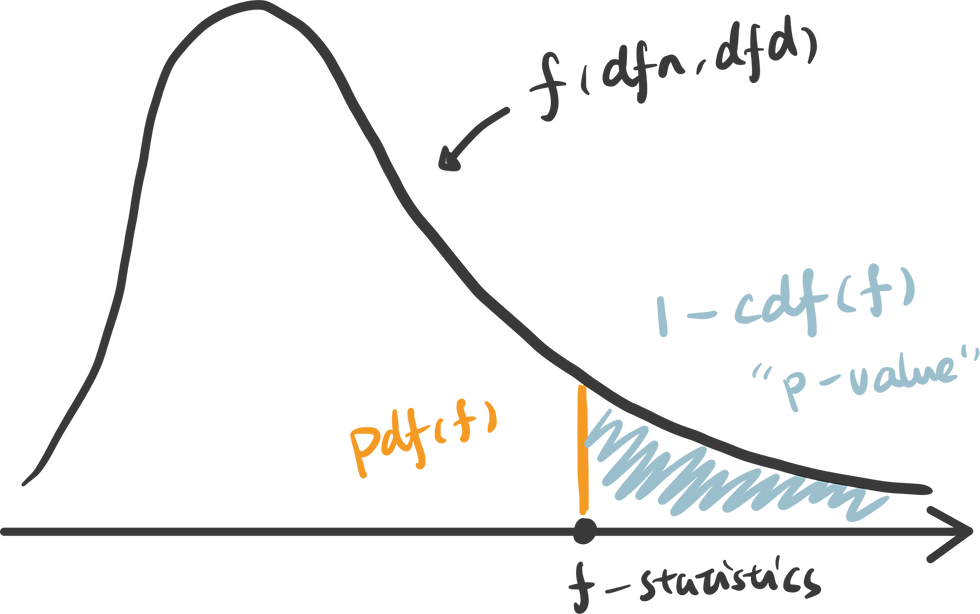
To easily get the f-statistics and p-value using Python, we can use the function stats.f_oneway() which returns p-value: 0.00040.

An interactive visualization of f-distribution with f-statistics vs. significance level. (Check out the code in our Code Snippet section, if you want to build this yourself. )

4. determine the statistical significance : Compare the p-value against the significance level 0.05, we can infer that there is strong evidence against the null hypothesis and very likely that there is difference in “NumWebPurchases” between at least two groups.

Chi-Squared Test

Chi-Squared test is for testing the relationship between two categorical variables. The underlying principle is that if two categorical variables are independent, then one categorical variable should have similar composition when the other categorical variable change. Let’s look at the example of whether “Education” and “Response” are independent.

First, use stacked bar chart and contingency table to summary the count of each category.

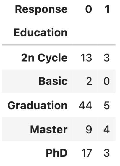
If these two variables are completely independent to each other (null hypothesis is true), then the proportion of positive Response and negative Response should be the same across all Education groups. It seems like composition are slightly different, but is it significant enough to say there is dependency - let’s run a Chi-Squared test.

null hypothesis: “Education” and “Response” are independent to each other.

alternative hypothesis: “Education” and “Response” are dependent to each other.

2. choose the appropriate test: Chi-Squared test is chosen and you probably found a pattern here, that Chi-distribution is also determined by the degree of freedom which is (row - 1) x (column - 1).

3. calculate the p-value: p value is calculated as the right tail cumulative area: 1 - rv.cdf(x).

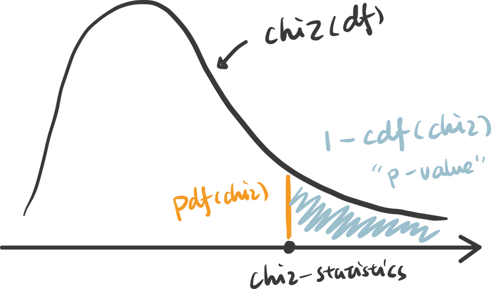
Python also provides a useful function to get the chi statistics and p-value given the contingency table.

An interactive visualization of chi-distribution with chi-statistics vs. significance level. (Check out the code in our Code Snippet section, if you want to build this yourself. )

4. determine the statistical significanc e: the p-value here is 0.41, suggesting that it is not statistical significant. Therefore, we cannot reject the null hypothesis that these two categorical variables are independent. This further indicates that “Education” may not be a strong predictor of “Response”.

Thanks for reaching so far, we have covered a lot of contents in this article but still have two important hypothesis tests that are worth discussing separately in upcoming posts.

z-test: test the difference between two categories of numeric variables - when sample size is LARGE

correlation: test the relationship between two numeric variables

Hope you found this article helpful. If you’d like to support my work and see more articles like this, treat me a coffee ☕️ by signing up Premium Membership with $10 one-off purchase.

Take home message.

In this article, we interactively explore and visualize the difference between three common statistical tests: t-test, ANOVA test and Chi-Squared test. We also use examples to walk through essential steps in hypothesis testing:

1. define the null and alternative hypothesis

2. choose the appropriate test

3. calculate the p-value

4. determine the statistical significance

• Data Science

Recent Posts

How to Self Learn Data Science in 2022

• Python Basics
• Interview Questions
• Python Quiz
• Popular Packages
• Python Projects
• Practice Python
• AI With Python
• Learn Python3
• Python Automation
• Python Web Dev
• DSA with Python
• Python OOPs
• Dictionaries
• Python - Pearson Correlation Test Between Two Variables
• How to create a Triangle Correlation Heatmap in seaborn - Python?
• Pearson Correlation Testing in R Programming
• How to plot the coherence between two signals in Python?
• How to Perform a Brown – Forsythe Test in Python
• Python | Kendall Rank Correlation Coefficient
• Sort Correlation Matrix in Python
• How to Perform a Mann-Kendall Trend Test in Python
• How to Calculate Rolling Correlation in Python?
• sympy.stats.variance() function in Python
• Python | Calculate Distance between two places using Geopy
• How to Perform an F-Test in Python
• How to detect whether a Python variable is a function?
• How to Calculate Correlation Between Two Columns in Pandas?
• Plotting Correlation Matrix using Python
• Python - Pearson's Chi-Square Test
• How to Calculate Correlation Between Multiple Variables in R?
• How to calculate the Pearson’s Correlation Coefficient?
• Difference between Correlation and Regression
• Create a correlation Matrix using Python

Python – Pearson Correlation Test Between Two Variables

What is correlation test?   The strength of the association between two variables is known as correlation test.  For instance, if we are interested to know whether there is a relationship between the heights of fathers and sons, a correlation coefficient can be calculated to answer this question. For know more about correlation please refer this. Methods for correlation analyses:   

• Parametric Correlation : It measures a linear dependence between two variables (x and y) is known as a parametric correlation test because it depends on the distribution of the data.
• Non-Parametric Correlation: Kendall(tau) and Spearman(rho) , which are rank-based correlation coefficients, are known as non-parametric correlation.

Note: The most commonly used method is the Parametric correlation method. Pearson Correlation formula:   

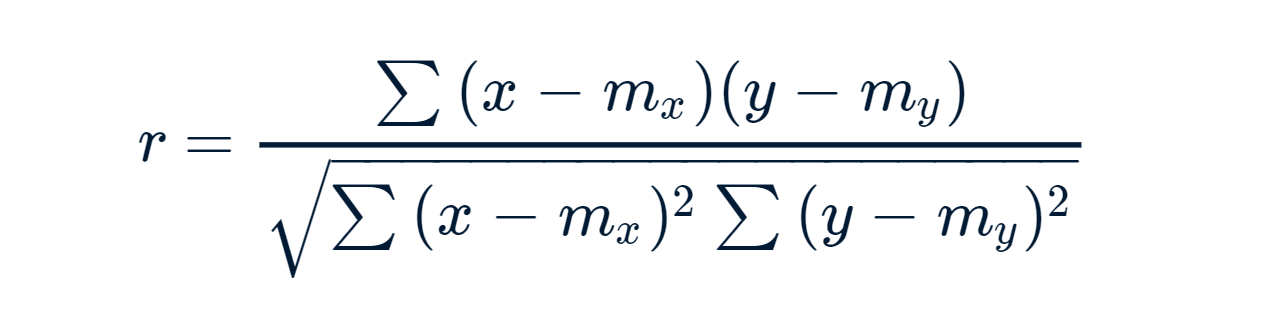
x and y are two vectors of length n  m, x and m, y corresponds to the means of x and y, respectively.

• r takes value between -1 (negative correlation) and 1 (positive correlation).
• r = 0 means no correlation.
• Can not be applied to ordinal variables.
• The sample size should be moderate (20-30) for good estimation.
• Outliers can lead to misleading values means not robust with outliers.

To compute Pearson correlation in Python – pearsonr() function can be used.  Python functions    

Syntax:   pearsonr(x, y) Parameters:  x, y: Numeric vectors with the same length   

Data: Download the csv file here. Code: Python code to find the pearson correlation    

Pearson Correlation for Anscombe’s Data:   Anscombe’s data also known as Anscombe’s quartet comprises of four datasets that have nearly identical simple statistical properties, yet appear very different when graphed. Each dataset consists of eleven (x, y) points. They were constructed in 1973 by the statistician Francis Anscombe to demonstrate both the importance of graphing data before analyzing it and the effect of outliers on statistical properties. Those 4 sets of 11 data-points are given here. Please download the csv file here.   When we plot those points it looks like this. I am considering 3 sets of 11 data-points here.   

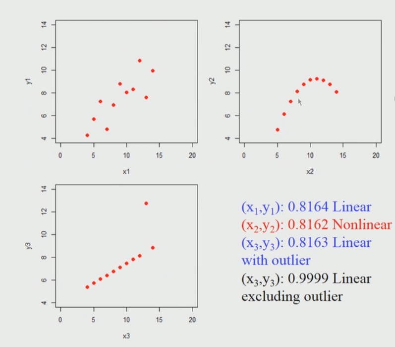
Brief explanation of the above diagram:   So, if we apply Pearson’s correlation coefficient for each of these data sets we find that it is nearly identical, it does not matter whether you actually apply into a first data set (top left) or second data set (top right) or the third data set (bottom left).  So, what it seems to indicate is that if we apply the Pearson’s correlation and we find the high correlation coefficient close to one in this first data set(top left) case. The key point is here we can’t conclude immediately that if the Pearson correlation coefficient is going to be high then there is a linear relationship between them, for example in the second data set(top right) this is a non-linear relationship and still gives rise to a high value.  

Please Login to comment...

Similar reads.

• data-science

Improve your Coding Skills with Practice

What kind of Experience do you want to share?

Raphael Vallat, PhD

Senior ML data scientist Oura Ring

Correlation(s) in Python

In this tutorial, you will learn how to calculate correlation between two or more variables in Python, using my very own Pingouin package .

Installation

To install Pingouin, you need to have Python 3 installed on your computer. If you are using a Mac or Windows, I strongly recommand installing Python via the Anaconda distribution . To install pingouin, just open a terminal and type the following lines:

Correlation coefficient

Load the data.

• Download the data and Jupyter notebook
• O penness to experience (inventive/curious vs. consistent/cautious)
• C onscientiousness (efficient/organized vs. easy-going/careless)
• E xtraversion (outgoing/energetic vs. solitary/reserved)
• A greeableness (friendly/compassionate vs. challenging/detached)
• N euroticism (sensitive/nervous vs. secure/confident)

Simple correlation between two columns

First, let's start by calculating the correlation between two columns of our dataframe. For instance, let's calculate the correlation between height and weight...Well, this is definitely not the most exciting research idea, but certainly one of the most intuitive to understand! For the sake of statistical testing, our hypothesis here will be that weight and height are indeed correlated. In other words, we expect that the taller someone is, the larger his/her weight is, and vice versa. This can be done simply by calling the pingouin.corr function:

• n is the sample size, i.e. how many observations were included in the calculation of the correlation coefficient
• r is the correlation coefficient, 0.45 in that case, which is quite high.
• CI95% are the 95% confidence intervals around the correlation coefficient
• r2 and adj_r2 are the r-squared and ajusted r-squared respectively. As its name implies, it is simply the squared r , which is a measure of the proportion of the variance in the first variable that is predictable from the second variable.
• p-val is the p-value of the test. The general rule is that you can reject the hypothesis that the two variables are not correlated if the p-value is below 0.05, which is the case. We can therefore say that there is a significant correlation between the two variables.
• BF10 is the Bayes Factor of the test, which also measure the statistical significance of the test. It directly measures the strength of evidence in favor of our initial hypothesis that weight and height are correlated. Since this value is very large, it indicates that there is very strong evidence that the two variables are indeed correlated. While they are conceptually different, the Bayes Factor and p-values will in practice often reach the same conclusion.
• power is the achieved power of the test, which is the likelihood that we will detect an effect when there is indeed an effect there to be detected. The higher this value is, the more robust our test is. In that case, a value of 1 means that we can be greatly confident in our ability to detect the significant effect.

How does the correlation look visually? Let's plot this correlation using the Seaborn package :

Pairwise correlation between several columns at once

What about the correlation between all the other columns in our dataframe? It would be a bit tedious to manually calculate the correlation between each pairs of columns in our dataframe (= pairwise correlation). Fortunately, Pingouin has a very convenient pairwise_corr function:

For simplicity, we only display the the most important columns and the most significant correlation in descending order. This is done by sorting the output table on the p-value column (lowest p-value first) and using .head() to only display the first rows of the sorted table. The pairwise_corr function is very flexible and has several optional arguments. To illustrate that, the code below shows how to calculate the non-parametric Spearman correlation coefficient (which is more robust to outliers in the data) on a subset of columns:

One can also easily calculate a one-vs-all correlation, as illustrated in the code below.

There are many more facets to the pairwise_corr function, and this was just a short introduction. If you want to learn more, please refer to Pingouin's documentation and the example Jupyter notebook on Pingouin's GitHub page.

Correlation matrix

As the number of columns increase, it can become really hard to read and interpret the ouput of the pairwise_corr function. A better alternative is to calculate, and eventually plot, a correlation matrix. This can be done using Pandas and Seaborn:

The only issue with these functions, however, is that they do not return the p-values, but only the correlation coefficients. Here again, Pingouin has a very convenient function that will show a similar correlation matrix with the r-value on the lower triangle and p-value on the upper triangle:

Now focusing on a subset of columns, and highlighting the significant correlations with stars:

• © Raphael Vallat
• Design: HTML5 UP
• Banner image: Nicholas Roerich

scipy.stats.permutation_test #

Performs a permutation test of a given statistic on provided data.

For independent sample statistics, the null hypothesis is that the data are randomly sampled from the same distribution. For paired sample statistics, two null hypothesis can be tested: that the data are paired at random or that the data are assigned to samples at random.

Contains the samples, each of which is an array of observations. Dimensions of sample arrays must be compatible for broadcasting except along axis .

Statistic for which the p-value of the hypothesis test is to be calculated. statistic must be a callable that accepts samples as separate arguments (e.g. statistic(*data) ) and returns the resulting statistic. If vectorized is set True , statistic must also accept a keyword argument axis and be vectorized to compute the statistic along the provided axis of the sample arrays.

The type of permutations to be performed, in accordance with the null hypothesis. The first two permutation types are for paired sample statistics, in which all samples contain the same number of observations and observations with corresponding indices along axis are considered to be paired; the third is for independent sample statistics.

'samples' : observations are assigned to different samples but remain paired with the same observations from other samples. This permutation type is appropriate for paired sample hypothesis tests such as the Wilcoxon signed-rank test and the paired t-test.

'pairings' : observations are paired with different observations, but they remain within the same sample. This permutation type is appropriate for association/correlation tests with statistics such as Spearman’s \(\rho\) , Kendall’s \(\tau\) , and Pearson’s \(r\) .

'independent' (default) : observations are assigned to different samples. Samples may contain different numbers of observations. This permutation type is appropriate for independent sample hypothesis tests such as the Mann-Whitney \(U\) test and the independent sample t-test.

Please see the Notes section below for more detailed descriptions of the permutation types.

If vectorized is set False , statistic will not be passed keyword argument axis and is expected to calculate the statistic only for 1D samples. If True , statistic will be passed keyword argument axis and is expected to calculate the statistic along axis when passed an ND sample array. If None (default), vectorized will be set True if axis is a parameter of statistic . Use of a vectorized statistic typically reduces computation time.

Number of random permutations (resamples) used to approximate the null distribution. If greater than or equal to the number of distinct permutations, the exact null distribution will be computed. Note that the number of distinct permutations grows very rapidly with the sizes of samples, so exact tests are feasible only for very small data sets.

The number of permutations to process in each call to statistic . Memory usage is O( batch * n ), where n is the total size of all samples, regardless of the value of vectorized . Default is None , in which case batch is the number of permutations.

The alternative hypothesis for which the p-value is calculated. For each alternative, the p-value is defined for exact tests as follows.

'greater' : the percentage of the null distribution that is greater than or equal to the observed value of the test statistic.

'less' : the percentage of the null distribution that is less than or equal to the observed value of the test statistic.

'two-sided' (default) : twice the smaller of the p-values above.

Note that p-values for randomized tests are calculated according to the conservative (over-estimated) approximation suggested in [2] and [3] rather than the unbiased estimator suggested in [4] . That is, when calculating the proportion of the randomized null distribution that is as extreme as the observed value of the test statistic, the values in the numerator and denominator are both increased by one. An interpretation of this adjustment is that the observed value of the test statistic is always included as an element of the randomized null distribution. The convention used for two-sided p-values is not universal; the observed test statistic and null distribution are returned in case a different definition is preferred.

The axis of the (broadcasted) samples over which to calculate the statistic. If samples have a different number of dimensions, singleton dimensions are prepended to samples with fewer dimensions before axis is considered.

numpy.random.RandomState }, optional

Pseudorandom number generator state used to generate permutations.

If random_state is None (default), the numpy.random.RandomState singleton is used. If random_state is an int, a new RandomState instance is used, seeded with random_state . If random_state is already a Generator or RandomState instance then that instance is used.

An object with attributes:

The observed test statistic of the data.

The p-value for the given alternative.

The values of the test statistic generated under the null hypothesis.

The three types of permutation tests supported by this function are described below.

Unpaired statistics ( permutation_type='independent' ):

The null hypothesis associated with this permutation type is that all observations are sampled from the same underlying distribution and that they have been assigned to one of the samples at random.

Suppose data contains two samples; e.g. a, b = data . When 1 < n_resamples < binom(n, k) , where

k is the number of observations in a ,

n is the total number of observations in a and b , and

binom(n, k) is the binomial coefficient ( n choose k ),

the data are pooled (concatenated), randomly assigned to either the first or second sample, and the statistic is calculated. This process is performed repeatedly, permutation times, generating a distribution of the statistic under the null hypothesis. The statistic of the original data is compared to this distribution to determine the p-value.

When n_resamples >= binom(n, k) , an exact test is performed: the data are partitioned between the samples in each distinct way exactly once, and the exact null distribution is formed. Note that for a given partitioning of the data between the samples, only one ordering/permutation of the data within each sample is considered. For statistics that do not depend on the order of the data within samples, this dramatically reduces computational cost without affecting the shape of the null distribution (because the frequency/count of each value is affected by the same factor).

For a = [a1, a2, a3, a4] and b = [b1, b2, b3] , an example of this permutation type is x = [b3, a1, a2, b2] and y = [a4, b1, a3] . Because only one ordering/permutation of the data within each sample is considered in an exact test, a resampling like x = [b3, a1, b2, a2] and y = [a4, a3, b1] would not be considered distinct from the example above.

permutation_type='independent' does not support one-sample statistics, but it can be applied to statistics with more than two samples. In this case, if n is an array of the number of observations within each sample, the number of distinct partitions is:

Paired statistics, permute pairings ( permutation_type='pairings' ):

The null hypothesis associated with this permutation type is that observations within each sample are drawn from the same underlying distribution and that pairings with elements of other samples are assigned at random.

Suppose data contains only one sample; e.g. a, = data , and we wish to consider all possible pairings of elements of a with elements of a second sample, b . Let n be the number of observations in a , which must also equal the number of observations in b .

When 1 < n_resamples < factorial(n) , the elements of a are randomly permuted. The user-supplied statistic accepts one data argument, say a_perm , and calculates the statistic considering a_perm and b . This process is performed repeatedly, permutation times, generating a distribution of the statistic under the null hypothesis. The statistic of the original data is compared to this distribution to determine the p-value.

When n_resamples >= factorial(n) , an exact test is performed: a is permuted in each distinct way exactly once. Therefore, the statistic is computed for each unique pairing of samples between a and b exactly once.

For a = [a1, a2, a3] and b = [b1, b2, b3] , an example of this permutation type is a_perm = [a3, a1, a2] while b is left in its original order.

permutation_type='pairings' supports data containing any number of samples, each of which must contain the same number of observations. All samples provided in data are permuted independently . Therefore, if m is the number of samples and n is the number of observations within each sample, then the number of permutations in an exact test is:

Note that if a two-sample statistic, for example, does not inherently depend on the order in which observations are provided - only on the pairings of observations - then only one of the two samples should be provided in data . This dramatically reduces computational cost without affecting the shape of the null distribution (because the frequency/count of each value is affected by the same factor).

Paired statistics, permute samples ( permutation_type='samples' ):

The null hypothesis associated with this permutation type is that observations within each pair are drawn from the same underlying distribution and that the sample to which they are assigned is random.

Suppose data contains two samples; e.g. a, b = data . Let n be the number of observations in a , which must also equal the number of observations in b .

When 1 < n_resamples < 2**n , the elements of a are b are randomly swapped between samples (maintaining their pairings) and the statistic is calculated. This process is performed repeatedly, permutation times, generating a distribution of the statistic under the null hypothesis. The statistic of the original data is compared to this distribution to determine the p-value.

When n_resamples >= 2**n , an exact test is performed: the observations are assigned to the two samples in each distinct way (while maintaining pairings) exactly once.

For a = [a1, a2, a3] and b = [b1, b2, b3] , an example of this permutation type is x = [b1, a2, b3] and y = [a1, b2, a3] .

permutation_type='samples' supports data containing any number of samples, each of which must contain the same number of observations. If data contains more than one sample, paired observations within data are exchanged between samples independently . Therefore, if m is the number of samples and n is the number of observations within each sample, then the number of permutations in an exact test is:

Several paired-sample statistical tests, such as the Wilcoxon signed rank test and paired-sample t-test, can be performed considering only the difference between two paired elements. Accordingly, if data contains only one sample, then the null distribution is formed by independently changing the sign of each observation.

The p-value is calculated by counting the elements of the null distribution that are as extreme or more extreme than the observed value of the statistic. Due to the use of finite precision arithmetic, some statistic functions return numerically distinct values when the theoretical values would be exactly equal. In some cases, this could lead to a large error in the calculated p-value. permutation_test guards against this by considering elements in the null distribution that are “close” (within a relative tolerance of 100 times the floating point epsilon of inexact dtypes) to the observed value of the test statistic as equal to the observed value of the test statistic. However, the user is advised to inspect the null distribution to assess whether this method of comparison is appropriate, and if not, calculate the p-value manually. See example below.

Fisher. The Design of Experiments, 6th Ed (1951).

B. Phipson and G. K. Smyth. “Permutation P-values Should Never Be Zero: Calculating Exact P-values When Permutations Are Randomly Drawn.” Statistical Applications in Genetics and Molecular Biology 9.1 (2010).

M. D. Ernst. “Permutation Methods: A Basis for Exact Inference”. Statistical Science (2004).

B. Efron and R. J. Tibshirani. An Introduction to the Bootstrap (1993).

Suppose we wish to test whether two samples are drawn from the same distribution. Assume that the underlying distributions are unknown to us, and that before observing the data, we hypothesized that the mean of the first sample would be less than that of the second sample. We decide that we will use the difference between the sample means as a test statistic, and we will consider a p-value of 0.05 to be statistically significant.

For efficiency, we write the function defining the test statistic in a vectorized fashion: the samples x and y can be ND arrays, and the statistic will be calculated for each axis-slice along axis .

After collecting our data, we calculate the observed value of the test statistic.

Indeed, the test statistic is negative, suggesting that the true mean of the distribution underlying x is less than that of the distribution underlying y . To determine the probability of this occurring by chance if the two samples were drawn from the same distribution, we perform a permutation test.

The probability of obtaining a test statistic less than or equal to the observed value under the null hypothesis is 0.4329%. This is less than our chosen threshold of 5%, so we consider this to be significant evidence against the null hypothesis in favor of the alternative.

Because the size of the samples above was small, permutation_test could perform an exact test. For larger samples, we resort to a randomized permutation test.

The approximate probability of obtaining a test statistic less than or equal to the observed value under the null hypothesis is 0.0225%. This is again less than our chosen threshold of 5%, so again we have significant evidence to reject the null hypothesis in favor of the alternative.

For large samples and number of permutations, the result is comparable to that of the corresponding asymptotic test, the independent sample t-test.

The permutation distribution of the test statistic is provided for further investigation.

Inspection of the null distribution is essential if the statistic suffers from inaccuracy due to limited machine precision. Consider the following case:

In this case, some elements of the null distribution differ from the observed value of the correlation coefficient r due to numerical noise. We manually inspect the elements of the null distribution that are nearly the same as the observed value of the test statistic.

If permutation_test were to perform the comparison naively, the elements of the null distribution with value 0.7999999999999999 would not be considered as extreme or more extreme as the observed value of the statistic, so the calculated p-value would be too small.

Instead, permutation_test treats elements of the null distribution that are within max(1e-14, abs(r)*1e-14) of the observed value of the statistic r to be equal to r .

This method of comparison is expected to be accurate in most practical situations, but the user is advised to assess this by inspecting the elements of the null distribution that are close to the observed value of the statistic. Also, consider the use of statistics that can be calculated using exact arithmetic (e.g. integer statistics).