define permanent income hypothesis

• Search Search Please fill out this field.

Permanent Income Hypothesis: Definition, How It Works, and Impact

Julia Kagan is a financial/consumer journalist and former senior editor, personal finance, of Investopedia.

Investopedia / Jiaqi Zhou

What Is the Permanent Income Hypothesis?

The permanent income hypothesis is a theory of consumer spending stating that people will spend money at a level consistent with their expected long-term average income . The level of expected long-term income then becomes thought of as the level of “permanent” income that can be safely spent. A worker will save only if their current income is higher than the anticipated level of permanent income, in order to guard against future declines in income.

Key Takeaways

• The permanent income hypothesis states that individuals will spend money at a level that is consistent with their expected long-term average income.
• Milton Friedman developed the permanent income hypothesis, believing that consumer spending is a result of estimated future income as opposed to consumption that is based on current after-tax income.
• Under the theory, if economic policies result in increased income, it will not necessarily translate into increased consumer spending.
• An individual's liquidity is a factor in their management of income and spending.

Understanding the Permanent Income Hypothesis

The permanent income hypothesis was formulated by the Nobel Prize-winning economist  Milton Friedman  in 1957. The hypothesis implies that changes in consumption behavior are not predictable because they are based on individual expectations. This has broad implications concerning economic policy.

Under this theory, even if economic policies are successful in increasing income in the economy, the policies may not kick off a multiplier effect in regards to increased consumer spending. Rather, the theory predicts that there will not be an uptick in consumer spending until workers reform expectations about their future incomes.

Milton believed that people will consume based on an estimate of their future income as opposed to what Keynesian economics proposed; people will consume based on their in the moment after-tax income. Milton's basis was that individuals prefer to smooth their consumption rather than let it bounce around as a result of short-term fluctuations in income.

Spending Habits Under the Permanent Income Hypothesis

If a worker is aware that they are likely to receive an income bonus at the end of a particular pay period, it is plausible that the worker’s spending in advance of that bonus may change in anticipation of the additional earnings. However, it is also possible that workers may choose to not increase their spending based solely on a short-term windfall. They may instead make efforts to increase their savings, based on the expected boost in income.

Something similar can be said of individuals who are informed that they are to receive an inheritance . Their personal expenditures could change to take advantage of the anticipated influx of funds, but per this theory, they may maintain their current spending levels in order to save the supplemental assets. Or, they may seek to invest those supplemental funds to provide long-term growth of their money rather than spend it immediately on disposable products and services.

Liquidity and the Permanent Income Hypothesis

The liquidity of the individual can play a role in future income expectations. Individuals with no assets may already be in the habit of spending without regard to their income; current or future.

Changes over time, however—through incremental salary raises or the assumption of new long-term jobs that bring higher, sustained pay—can lead to changes in permanent income. With their expectations elevated, employees may allow their expenditures to scale up in turn.

• Terms of Service
• Editorial Policy
• Privacy Policy
• Your Privacy Choices

Financial Tips, Guides & Know-Hows

Home > Finance > Permanent Income Hypothesis: Definition, How It Works, And Impact

Permanent Income Hypothesis: Definition, How It Works, And Impact

Published: January 7, 2024

Learn about the Permanent Income Hypothesis in finance, its definition, how it works, and the impact it has on financial decision-making.

• Definition starting with P

(Many of the links in this article redirect to a specific reviewed product. Your purchase of these products through affiliate links helps to generate commission for LiveWell, at no extra cost. Learn more )

Unlocking the Secrets of the Permanent Income Hypothesis

When it comes to understanding personal finances, there are several theories and concepts that can help us make better decisions about saving and spending. One such theory that holds a key place in the world of financial planning is the Permanent Income Hypothesis (PIH). In this blog post, we will delve into the essence of PIH, how it works, and the impact it can have on our financial well-being.

Key Takeaways:

• Permanent Income Hypothesis (PIH) suggests that individuals base their current consumption on their long-term average income.
• Personal saving rates and spending patterns can vary based on the belief that income changes are often temporary and individuals attempt to smooth their consumption over time.

So, what exactly is the Permanent Income Hypothesis? Developed by Nobel laureate Milton Friedman in the late 1950s, PIH posits that individuals make consumption decisions based on their long-term average income rather than on short-term fluctuations. In other words, people tend to smooth out their consumption patterns over time, anticipating future income changes and adjusting their spending and saving habits accordingly.

According to Friedman, individuals perceive temporary changes in income as transitory and do not significantly impact their consumption behavior. Instead, they prioritize maintaining a consistent standard of living, which leads them to save during times of high income and borrow during periods of low income to achieve this equilibrium. Thus, the Permanent Income Hypothesis suggests that people’s spending decisions are determined by their permanent or long-term income expectations rather than their current income situation.

How does the Permanent Income Hypothesis work in practice? Let’s consider an example. Imagine you receive a substantial bonus at work. While it might be tempting to go on a spending spree, adhering to the principles of PIH would suggest that you save a significant portion of that bonus to smooth out any future income fluctuations. By saving instead of splurging, you are aligning your spending patterns with your long-term average income and prioritizing financial stability over short-term gratification.

Now, let’s explore the impact of the Permanent Income Hypothesis. Understanding and applying PIH can have several benefits for individuals and families:

• Improved Financial Planning: By considering long-term income expectations rather than temporary changes, individuals can better plan for their financial future and make more informed decisions regarding saving, investing, and budgeting.
• Reduced Financial Stress: Viewing changes in income as temporary can help individuals avoid panicking or overreacting during periods of financial instability. Instead, they can rely on the belief that their long-term income will eventually stabilize, enabling them to make sustainable financial choices.
• Increased Saving Rates: Since individuals base their consumption decisions on long-term income expectations, following the Permanent Income Hypothesis may encourage higher saving rates. This can result in a more secure financial position and provide a safety net during emergencies.

In conclusion, the Permanent Income Hypothesis offers valuable insights into how individuals make consumption decisions based on their long-term average income. By understanding and applying the principles of PIH, we can enhance our financial planning, reduce stress, and achieve a more stable and secure financial future. So, the next time you face a financial windfall or setback, consider the wisdom of the Permanent Income Hypothesis and make financial decisions that align with your long-term goals.

20 Quick Tips To Saving Your Way To A Million Dollars

Our Review on The Credit One Credit Card

How To Get Approved For An Apple Credit Card

How To Add Tradelines To Your Credit Report

Latest articles.

Navigating Crypto Frontiers: Understanding Market Capitalization as the North Star

Written By:

Financial Literacy Matters: Here’s How to Boost Yours

Unlocking Potential: How In-Person Tutoring Can Help Your Child Thrive

Understanding XRP’s Role in the Future of Money Transfers

Navigating Post-Accident Challenges with Automobile Accident Lawyers

Related post.

By:  •  Finance

Please accept our Privacy Policy.

We uses cookies to improve your experience and to show you personalized ads. Please review our privacy policy by clicking here .

• https://livewell.com/finance/permanent-income-hypothesis-definition-how-it-works-and-impact/

Milton Friedman's Permanent Income Hypothesis

Milton Friedman is the most influential economist of the last fifty years. He is, with John Maynard Keynes, perhaps even the most influential of the entire 20 th century .  His theories and research continue to shape public policy debates even until today.  One of his most important and lasting is the Permanent Income Hypothesis .

The Permanent Income Hypothesis

One of Friedman’s most influential and revolutionary theories was his challenge to the traditional Keynesian consumption function, which includes simple after-tax income as a variable in the consumption.

Friedman countered, that those who consume today take future taxes, price increases, salary increases, and other factors into account. This is summarized in his Permanent Income Hypothesis .

Defining the Permanent Income Hypothesis

More specifically, the Permanent Income Hypothesis argues that people consume based off of their overall estimation of future income . Economic thought at the time assumed people consumed only based on their current after-tax income.

For a simple example, consider a college student .

A college student borrows a lot of money to go into a (hopefully) moderate amount of debt. She does this expecting that her debt now will be easily covered by her increased earning power.

In this way, she "smoothes" her consumption, consuming only slightly less during college than immediately after. This is even after the huge increase in income.

Smoothing Consumption and Peak Earnings

Milton Friedman, who created the Permanent Income Hypothesis ( Wikipedia)

Let's look at it another way. A person is going to earn a certain amount of money in his lifetime.

In the framework  of the Permanent Income Hypothesis, he'll smooth his spending over a career based off of his expectations, as opposed to bouncing wildly around as raises and salary increases come.

On the other side of the scale is a near-retiree. Near-retirees are usually at a relative high point in their income. With kids out of the house, they usually save quite a bit in the expectation that their future "income" will decrease significantly to their level of Social Security payments). A cautious near-retiree carefully saves money to avoid an income shock when he is no longer earning active income.

These anecdotal examples are pretty strong examples of Milton Friedman’s hypothesis.

One clarifying remark before we move onto modern research on the topic:

All  consumption smoothing decisions are based only on readily available information. Obviously, you can't predict lottery winnings or stock market luck, so the Permanent Income Hypothesis doesn't account for these types of windfalls.

Why Does the Permanent Income Hypothesis Matter to the Economy?

The Permanent Income Hypothesis has significant implications for government entitlement programs. It is especially relevant for those who will continue working for quite a while, say a decade or more.

Let's say you're under the age of 45. If the government increases spending today, you might expect them to match it with an equal tax increase at some point in the near future. This means that the government's new spending will not in spur you to increase your short term spending – in fact, you might increase your savings rate in anticipation of higher taxes. This effect might go a long way – or the full way – towards cancelling out the effects of some government policies or lending programs.

Milton Friedman is known for this counter-example and counter-hypothesis to Keynes’ deficit-fueled recession-fighting formula. Friedman believed that monetary policy is the appropriate tool to fight recessions. Friedman stated lower rates in the near term eventually lead to an increase in short-term output at the cost of long-term inflation.

Problems and Tests for the Permanent Income Hypothesis

A major problem for the hypothesis hypothesis is the amount and quality of known information.

If you're 35 today, can you actually know how government spending now will lead to an increase in taxes for yourself later in your life?

Even if you do realize there will be a tax increase, will you change your consumption patterns perfectly to match?

Probably not, and further the effect will be different across the population. Perhaps the way citizens react to spending increases is really a blend between Keynes’ and Friedman’s hypotheses.

Testing the Hypothesis

One of the best papers testing the hypothesis is David Wilcox's “ Social Security Benefits, Consumption Expenditure, and the Life Cycle Hypothesis ” from the Journal of Political Economy in April, 1989. It looks at Social Security benefit increases in between 1974 and 1982.

Before 1974, increases in Social Security benefits for recipients were random and varied wildly. In 1974, however, a law was passed to link SS payment increases to increase in CPI.

Over the next eight years (and continuing today), the increase in Social Security benefits were announced around 2.5 months before they occurred.

This clearly directly tests the hypothesis. These are known increases in a Social Security recipient’s income. The Permenent Income Hypothesis predicts that retirees would increase consumption even before payments increase, effectively borrowing from future payments. Thus, there'd be a negligible, statistically insignificant change in spending habits before and after the actual payment increase.

There are a number of nuances in the paper, but suffice to say there was a rather large percentage increase in spending among retirees immediately after payment increases took place. Thus, you can conclude that the Permanent Income Effect, if it exists, was small in that population.

The Permanent Income Hypothesis Today

Obviously, we'll continue debating the proper policy response to help spur the economy during difficult times. Expect the Keynes versus Friedman debate of Monetary versus Fiscal policy to continue for quite some time.

NEWSLETTER  JOIN THE LIST

Popular  in the last week.

• Minutes Calculator: See How Many Minutes are Between Two Times
• Hours Calculator: See How Many Hours are Between Two Times
• Week Calculator: How Many Weeks Between Dates?
• Income Percentile Calculator for the United States
• Month Calculator: Number of Months Between Dates
• Height Percentile Calculator for Men and Women in the United States
• S&P 500 Return Calculator, with Dividend Reinvestment
• Years Calculator: How Many Years Between Two Dates
• Age Difference Calculator: Compute the Age Gap
• Household Income Percentile Calculator for the United States
• Income Percentile by Age Calculator for the United States
• Least to Greatest Calculator: Sort in Ascending Order
• Net Worth by Age Calculator for the United States
• Average, Median, Top 1%, and all United States Household Income Percentiles
• Net Worth Percentile Calculator for the United States
• Income Percentile by State Calculator
• Stock Total Return and Dividend Reinvestment Calculator (US)
• Bond Yield to Maturity (YTM) Calculator

CLASSICS  ON THE SITE

• Average, Median, Top 1%, and Income Percentile by City
• How Many Millionaires Are There in America?
• Stock Return Calculator, with Dividend Reinvestment
• Historical Home Prices: Monthly Median Value in the US
• Bond Pricing Calculator

Don't Quit Your Day Job...

5.1 The Permanent Income Hypothesis

The Permanent Income Hypothesis (PIH) attempts to explain consumption behavior and expected relationships in cross-sectional and longitudinal APC's by first redefining measures of income.

Observed values of aggregate income 'Y' can be divided up into two separate components: 'Y P ' Permanent (or projected levels of) Income and 'Y T ' Transitory (or unexpected changes in) Income. Thus:

Y = Y P + Y T .

The transitory component has an expected value of zero (E[Y T t ] = 0) reflecting the notion that over time transitory gains are offset by future transitory losses and vice-versa. Thus in the long run observed levels of income 'Y' are equal to permanent income 'Y P '.

Finally, according to the PIH consumption expenditure is proportional to permanent income:

such that the parameter ' k ', a constant, represents both the average propensity to consume and the marginal propensity to consume . This consumption function (as shown with the blue line below) is described more accurately as a long run consumption function consistent with the observed long run results of consumption behavior.

Observed short run behavior is explained through the value of transitory income for different income groups. Specifically, transitory income for low income groups is assumed to be negative reflecting the notion that over time transitory losses exceed transitory gains for this group of individuals:

Y T L < 0 → Y L < Y P L

For middle income groups the value of transitory income is equal to zero over time such that observed and permanent income take the same value:

Y T M = 0 → Y M = Y P M

Finally, for high income groups, transitory gains exceed transitory losses such that transitory income is on average positive over time or:

Y T H > 0 → Y H > Y P H

The impact of this transitory component can be used to develop a short run consumption function (the red line) as shown in the diagram.

The PIH provides a framework for understanding how households will likely react to changes in income in making near-term consumption spending decisions. If the changes in income are perceived to be transitory, consumption spending may be unaffected -- transitory gains will be saved to meet the demands of transitory losses sometime in the future. Changes in income that are perceived to be permanent can have a real and immediate impact on consumption spending.

Permanent-Income Hypothesis

• Reference work entry
• First Online: 01 January 2017
• pp 4886–4889
• Cite this reference work entry

• Mark Aguiar &
• Erik Hurst  

The permanent income hypothesis (PIH) is a theory that links an individual’s consumption at any point in time to that individual’s total income earned over their lifetime.

This is a preview of subscription content, log in via an institution to check access.

Access this chapter

Institutional subscriptions

Unable to display preview.  Download preview PDF.

Bibliography

Aguiar, M. and Hurst, E. (2005). Consumption vs. expenditure. Journal of Political Economy 113, 919–48.

Article   Google Scholar  

Aguiar, M. and Hurst, E. 2007. Lifecycle prices and production. American Economic Review . (forthcoming).

Google Scholar  

Attanasio, O. and Browning, M. (1995). Consumption over the life cycle and over the business cycle. American Economic Review 85, 1118–37.

Attanasio, O.P. and Weber, G. (1995). Is consumption growth consistent with intertemporal optimization? Evidence from the consumer expenditure survey. Journal of Political Economy 103, 1121–57.

Attanasio, O., Banks, J., Meghir, C. and Weber, G. (1999). Humps and bumps in lifetime consumption. Journal of Business and Economic Statistics 17, 22–35.

Becker, G. (1965). A theory of the allocation of time. Economic Journal 75, 493–508.

Bernheim, B.D., Skinner, J. and Weinberg, S. (2001). What accounts for the variation in retirement wealth among U.S. households? American Economic Review 91, 832–57.

Browning, M. and Collado, D. (2001). The response of expenditures to anticipated income changes: panel data estimates. American Economic Review 91, 681–92.

Carroll, C. (2001). A theory of the consumption function, with and without liquidity constraints. Journal of Economic Perspectives 15, 23–45.

Cochrane, J. (1991). A simple test of consumption insurance. Journal of Political Economy 99, 957–76.

Friedman, M. (1957) A Theory of the Consumption Function . (Princeton: Princeton University Press).

Gourinchas, P.-O. and Parker, J. (2002). Consumption over the life-cycle. Econometrica 70, 47–89.

Hall, R. (1978). Stochastic implications of the life cycle-permanent income hypothesis: theory and evidence. Journal of Political Economy 86, 971–87.

Hsieh, C.-T. (2003). Do consumers react to anticipated income changes? Evidence from the Alaska permanent fund. American Economic Review 93, 397–405.

Modigliani, E and Brumberg, R. 1954. Utility analysis and the consumption function: an interpretation of the cross section data. In Post-Keynesian Economics , ed. K. Kurihara. New Brunswick, NJ: Rutgers University Press.

Parker, J. (1999). The reaction of household consumption to predictable changes in payroll tax rates. American Economic Review 89, 959–73.

Shea, J. (1995). Union contracts and the life-cycle/permanent income hypothesis. American Economic Review 85, 186–200.

Souleles, N. (1999). The response of household consumption to income tax refunds. American Economic Review 89, 947–58.

Townsend, R. (1994). Risk and insurance in village India. Econometrica 62, 539–91.

Zeldes, S. (1989). Consumption and liquidity constraints: an empirical investigation. Journal of Political Economy 97, 305–46.

Download references

You can also search for this author in PubMed   Google Scholar

Editor information

Copyright information.

© 2008 Palgrave Macmillan, a division of Macmillan Publishers Limited

About this entry

Cite this entry.

Aguiar, M., Hurst, E. (2008). Permanent-Income Hypothesis. In: Durlauf, S.N., Blume, L.E. (eds) The New Palgrave Dictionary of Economics. Palgrave Macmillan, London. https://doi.org/10.1007/978-1-349-58802-2_1269

Download citation

DOI : https://doi.org/10.1007/978-1-349-58802-2_1269

Published : 17 August 2017

Publisher Name : Palgrave Macmillan, London

Print ISBN : 978-0-333-78676-5

Online ISBN : 978-1-349-58802-2

Share this entry

Anyone you share the following link with will be able to read this content:

Sorry, a shareable link is not currently available for this article.

Provided by the Springer Nature SharedIt content-sharing initiative

• Publish with us

Policies and ethics

• Find a journal
• Track your research

Quickonomics

Permanent Income Hypothesis

Definition of permanent income hypothesis.

The Permanent Income Hypothesis (PIH) is an economic theory that suggests individuals’ consumption patterns are determined by their long-term average income rather than their short-term fluctuations in income. According to this hypothesis, people adjust their consumption based on their expectations of future income rather than their current income level.

To illustrate the Permanent Income Hypothesis, consider two individuals: Alice and Bob. Alice is a salaried employee who earns a consistent income every month, while Bob is self-employed and experiences fluctuations in his income from month to month.

Alice, who has a stable income, consistently spends a portion of her income on necessities, such as rent, groceries, and utility bills. She also saves a portion for future expenses and retirement. Even if Alice’s income increases or decreases slightly from month to month, her overall consumption and saving habits remain relatively stable because her long-term average income remains constant.

On the other hand, Bob’s income is more volatile as a self-employed individual. When Bob has a month with high earnings, he spends more on luxury items and experiences. However, during months with lower income, he reduces his discretionary spending to compensate for the decrease in earnings.

This example demonstrates how individuals with different income patterns respond differently to changes in income. Alice’s consumption is more closely linked to her long-term average income, while Bob’s consumption fluctuates with his short-term income.

Why the Permanent Income Hypothesis Matters

The Permanent Income Hypothesis has important implications for economic policy and the understanding of consumer behavior. If the hypothesis holds true, it suggests that policies aimed at stimulating short-term consumption, such as temporary tax cuts or government transfers, may have limited long-term effects. Instead, policies that focus on promoting long-term income growth, such as investments in education and infrastructure, may have a more significant impact on consumption and economic well-being.

Understanding the Permanent Income Hypothesis also helps to explain why individuals may be hesitant to significantly increase their consumption even when their current income rises temporarily, such as receiving a year-end bonus. Instead, they may choose to save or invest the extra income, anticipating future fluctuations or planning for long-term goals.

Overall, the Permanent Income Hypothesis provides a framework for analyzing patterns of consumption and saving behavior, allowing economists and policymakers to make more informed decisions regarding income inequality, social welfare programs, and economic stability.

To provide the best experiences, we and our partners use technologies like cookies to store and/or access device information. Consenting to these technologies will allow us and our partners to process personal data such as browsing behavior or unique IDs on this site and show (non-) personalized ads. Not consenting or withdrawing consent, may adversely affect certain features and functions.

Click below to consent to the above or make granular choices. Your choices will be applied to this site only. You can change your settings at any time, including withdrawing your consent, by using the toggles on the Cookie Policy, or by clicking on the manage consent button at the bottom of the screen.

The Permanent Income Hypothesis

MARC RIS BibTeΧ

Download Citation Data

More from NBER

In addition to working papers , the NBER disseminates affiliates’ latest findings through a range of free periodicals — the NBER Reporter , the NBER Digest , the Bulletin on Retirement and Disability , the Bulletin on Health , and the Bulletin on Entrepreneurship  — as well as online conference reports , video lectures , and interviews .

Permanent Income Hypothesis

• Post author: Viren Rehal
• Post published: August 16, 2022
• Post category: Consumption function / Macroeconomics
• Post comments: 0 Comments

Empirical studies and observations exposed the shortcomings of the absolute income hypothesis . It failed to explain the patterns of consumption over a long period of time. It did not consider the role of business cycles or wealth as a factor in determining consumption. As a result, several other theories emerged which attempted to explain the behaviour of consumption, such as the Permanent Income Hypothesis.

Permanent income and consumption

The permanent income hypothesis was introduced by Milton Friedman. It is based on the assumption that individuals aim for utility maximization. According to Friedman, permanent consumption is a function of the permanent income of a consumer.

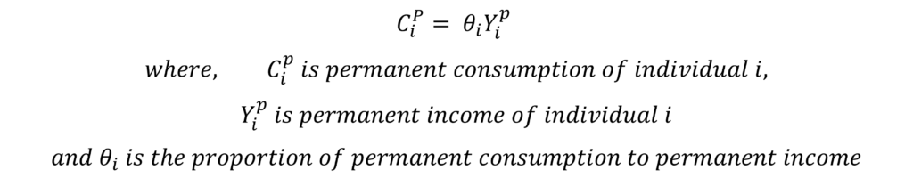
Here, “ theta ” explains the proportion of permanent income used in permanent consumption, which turns out to be simply the ratio of permanent consumption to the permanent income of the consumer. The actual value of this ratio depends on several factors including the rate of interest, tastes and preferences of the given consumer and expected income.

Relationship between permanent and total income/consumption

This permanent income and permanent consumption are different from total income and total consumption in a given time period. The relationship between these can be illustrated as follows:

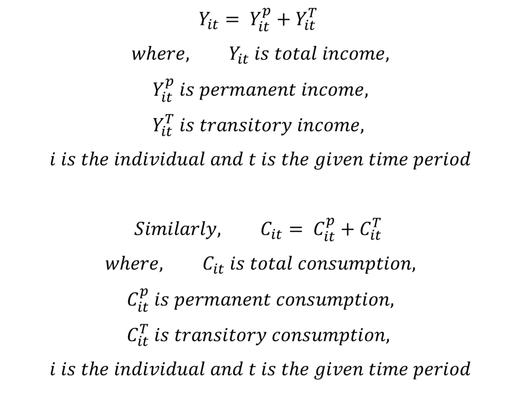
The transitory income and transitory consumption are random deviations from permanent income and permanent consumption respectively, which leads to differences in total income and consumption. This transitory income and consumption can be positive, negative or zero. The sum of transitory and permanent elements makes up the total income and consumption in a given time period for each individual.

assumptions made by Friedman

Friedman made some assumptions about all the above components and the way they are related to each other. These assumptions help explain the behaviour of consumption and can be stated as follows:

• There is no relationship between transitory income and permanent income. Hence, total income fluctuates randomly around the permanent income with zero covariance between the total and permanent income of different individuals.
• Similarly, there is no correlation between transitory consumption and permanent consumption. Total consumption is a random fluctuation around permanent consumption. Therefore, the covariance between total and permanent consumption is zero.
• There is no relationship between transitory income and transitory consumption. The covariance of transitory income and transitory consumption is zero. This is true because Friedman includes the purchase of non-durable goods only and not the purchase of durable goods in consumption. The usage of durable goods is included in consumption through depreciation. Therefore, if consumers purchase durable goods from transitory income, it does not have a significant effect on consumption because only usage of durables is included in consumption, not their purchase.

Empirical Evidence and explanation using Permanent Income Hypothesis

Mpc < apc in cross-sectional studies.

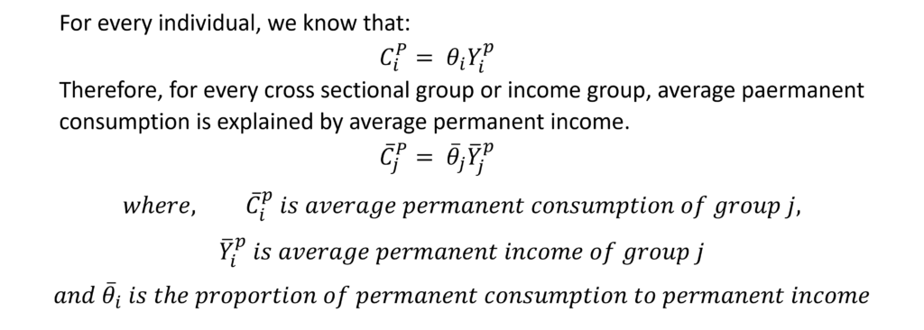
However, transitory consumption has no relationship with transitory income or permanent consumption. The average transitory consumption of every income group will be zero. As a result, average permanent consumption will be equal to average total consumption in every income group.

An income group ‘b’, which has an average income higher than the average population income, will have a positive average transitory income. That is, the average permanent income of that group will be less than the average total income. This difference is equal to the value of average transitory income. Since the average transitory consumption will be zero, the average permanent and average total consumption of group ‘b’ will be equal. It is shown by point “B” in the diagram.

On the other hand, income group ‘a’ has a negative average transitory income implying that the average permanent income is greater than the average total income in that case. The average total and average permanent consumption will be equal, corresponding to point A.

Similarly, the income group with an average income equal to the average population income has zero transitory income. At this point, the average permanent income is equal to the average total income of the group.

Cross-sectional consumption function

This gives rise to the cross-sectional consumption function which is shown by ‘C’. In the case of high-income group ‘b’, APC is observed at point B. Point B lies below the population consumption line, hence, APC at point B is less than the overall APC of the population which is equal to theta . Conversely, APC at point A corresponding to group ‘a’ lies higher than the population consumption line. APC is greater than the constant APC of the population (theta). Hence, APC is falling as we move from low to high-income groups and MPC<APC on the consumption function ‘C’. The slope of the cross-sectional consumption function is less than the population consumption line.

As the economy grows and average permanent income rises for all groups, this consumption function ‘C’ keeps shifting upwards along the trend, which is the population consumption line. In the long run, the observed consumption function is the population consumption line of “ theta ” with a constant APC.

Long-run and cyclical fluctuations

The explanation of consumption over a long run and short run fluctuation due to business cycles is similar to that of cross-sectional groups.

Instead of the high-income group, we have a period of boom in the economy at point B when the average transitory income is positive. The average permanent income is, therefore, less than the average total income in the economy. On the opposite end, we have a period of slump in the economy at point A. Average transitory income is negative and average permanent income is greater than the average total income in the economy.

These points A and B corresponding to periods of slump and boom, show us the short-run consumption function ‘C’. At point A, APC is greater than long-run APC ( theta ) and APC at point B is less than long-run APC. Therefore, MPC < APC in the short run corresponds to each business cycle when the slope of ‘C‘ is less than the trend line. The long-run consumption is shown by the trend line with APC = MPC at constant theta . This trend line or long-run permanent consumption is observed over a long period as the economy grows and the short-run consumption function goes on shifting upwards.

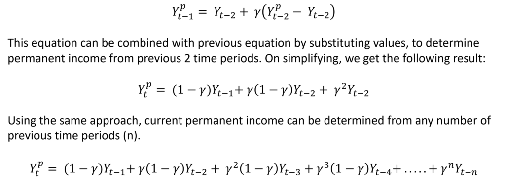
determining permanent income: adaptive expectations

This approach by Friedman divides total income into permanent income and transitory income. In reality, these two components are not observed separately, but, only the total income is observed. Therefore, Friedman used the method of adaptive expectations to separate permanent income from transitory income. Using adaptive expectation, permanent income can be extracted from total income in actual time series data as follows:

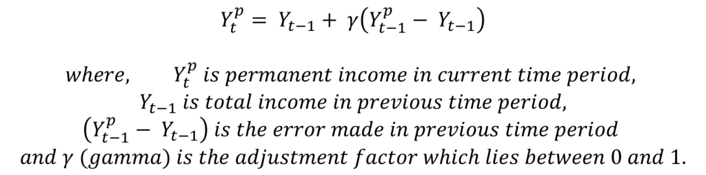
Therefore, if gamma is closer to zero, it implies that we are giving less weightage to the last period error (transitory income) and relying more on the actual income in the previous time period. On the contrary, if gamma is close to 1, we are giving high weightage to the error in determining permanent income. At gamma = 0, we completely ignore the past error. At gamma = 1, we don’t change expectations at all as we assume error will be exactly the same as last period.

The above equation shows that the permanent income in the current period depends only on past incomes. Similarly, permanent income in the previous time period (t-1) can be expressed as follows:

criticism of Permanent Income Hypothesis

• It does not explicitly account for wealth or the role of assets. It implicitly includes assets as part of consumption through the ‘usage’ of assets, measured by depreciation and rate of interest.
• In adaptive expectations, only previous period income is used to determine current permanent income. Whereas, income is a function of many factors apart from previous incomes.
• It includes the consumption of durables only through depreciation and rate of interest. The purchase of durables from transitory income or windfall gains is not considered.
• The theory assumes APC to be constant at “ theta ” while estimating permanent consumption. However, it does not have to be constant even within an income group. APC is expected to fall as income increases because lower-income groups have to spend a greater portion of their income to meet their needs.

You Might Also Like

Accelerator theory and its process, relative income hypothesis, absolute income hypothesis, leave a reply cancel reply.

To provide the best experiences, we and our partners use technologies like cookies to store and/or access device information. Consenting to these technologies will allow us and our partners to process personal data such as browsing behavior or unique IDs on this site and show (non-) personalized ads. Not consenting or withdrawing consent, may adversely affect certain features and functions.

Click below to consent to the above or make granular choices. Your choices will be applied to this site only. You can change your settings at any time, including withdrawing your consent, by using the toggles on the Cookie Policy, or by clicking on the manage consent button at the bottom of the screen.

Absolute, Relative and Permanent Income Hypothesis (With Diagram)

1. Absolute Income Hypothesis:

Keynes’ consumption function has come to be known as the ‘absolute income hypothesis’ or theory. His statement of the relationship be­tween income and consumption was based on the ‘fundamental psychological law’.

He said that consumption is a stable function of cur­rent income (to be more specific, current dis­posable income—income after tax payment).

Because of the operation of the ‘psychological law’, his consumption function is such that 0 < MPC < 1 and MPC < APC. Thus, a non- proportional relationship (i.e., APC > MPC) between consumption and income exists in the Keynesian absolute income hypothesis. His consumption function may be rewritten here with the form

C = a + bY, where a > 0 and 0 < b < 1.

ADVERTISEMENTS:

It may be added that all the characteristics of Keynes’ consumption function are based not on any empirical observation, but on ‘fun­damental psychological law’, i.e., experience and intuition.

(i) Consumption Function in the Light of Empirical Observations:

Meanwhile, at­tempts were made by the empirically-oriented economists in the late 1930s and early 1940s for testing the conclusions made in the Keynesian consumption function.

(ii) Short Run Budget Data and Cyclical Data:

Let us consider first the budget studies data or cross-sectional data of a cross section of the population and then time-series data. The first set of evidence came from budget studies for the years 1935-36 and 1941-42. These budget studies seemed consistent with the Keynes’ own conclusion on consumption-income relationship. The time-series data of the USA for the years 1929-44 also gave reasonably good support to the Keynesian theoretical consumption function.

Since the time period covered is not long enough, this empirical consumption function derived from the time- series data for 1929-44 may be called ‘cyclical’ consumption function. Anyway, we may conclude now that these two sets of data that generated consumption function consistent with the Keynesian consumption equation, C = a + bY.

Further, 0 < b < 1 and AMC < APC.

(iii) Long Run Time-Series Data:

However, Simon Kuznets (the 1971 Nobel prize winner in Economics) considered a long period cov­ering 1869 to 1929. His data may be described as the long run or secular time-series data. This data indicated no long run change in con­sumption despite a very large increase in in­come during the said period. Thus, the long run historical data that generated long run or secular consumption function were inconsist­ent with the Keynesian consumption function.

From Kuznets’ data what is obtained is that:

(a) There is no autonomous consumption, i.e., ‘a’ term of the consumption function and

(b) A proportional long run consumption func­tion in which APC and MPC are not different. In other words, the long run consumption function equation is C = bY.

As a = 0, the long run consumption func­tion is one in which APC does not change over time and MPC = APC at all levels of income as contrasted to the short run non-propor­tional (MPC < APC) consumption-income re­lationship. Being proportional, the long run consumption function starts form the origin while a non-proportional short run consump­tion function starts from point above the ori­gin. Keynes, in fact, was concerned with the long run situation.

But what is baffling and puzzling to us that the empirical studies suggest two different consumption functions a non-proportional cross-section function and a proportional long run time-series function.

2. Relative Income Hypothesis:

Studies in consumption then were directed to resolve the apparent conflict and inconsistencies between Keynes’ absolute income hy­pothesis and observations made by Simon Kuznets. Former hypothesis says that in the short run MPC < APC, while Kuznets’ obser­vations say that MPC = APC in the long run.

One of the earliest attempts to offer a reso­lution of the conflict between short run and long run consumption functions was the ‘rela­tive income hypothesis’ (henceforth R1H) of ).S. Duesenberry in 1949. Duesenberry be­lieved that the basic consumption function was long run and proportional. This means that average fraction of income consumed does not change in the long run, but there may be variation between consumption and in­come within short run cycles.

Duesenberry’s RIH is based on two hypotheseis first is the relative income hy­pothesis and second is the past peak income hypothesis.

Duesenberry’s first hypothesis says that consumption depends not on the ‘absolute’ level of income but on the ‘relative’ income— income relative to the income of the society in which an individual lives. It is the relative position in the income distribution among families influences consumption decisions of individuals.

A households consumption is determined by the income and expenditure pattern of his neighbours. There is a tendency on the part of the people to imitate or emulate the consumption standards maintained by their neighbours. Specifically, people with relatively low incomes attempt to ‘keep up with the Joneses’—they consume more and save less. This imitative or emulative nature of consumption has been described by Duesenberry as the “demonstration effect.”

The outcome of this hypothesis is that the individuals’ APC depends on his relative position in income distribution. Families with relatively high incomes experience lower APCs and families with relatively low incomes experience high APCs. If, on the other hand, income distribution is relatively constant (i.e., keeping each families relative position unchanged while incomes of all families rise). Duesenberry then argues that APC will not change.

Thus, in the aggregate we get a proportional relationship between aggregate income and aggregate consumption. Note MPC = APC. Hence the R1H says that there is no apparent conflict between the results of cross-sectional budget studies and the long run aggregate time-series data.

In terms of the second hypothesis short run cyclical behaviour of the Duesenberry’s aggregate consumption function can be explained. Duesenberry hypothesised that the present consumption of the families is influenced not just by current incomes but also by the levels of past peak incomes, i.e., C = f(Y ri , Y pi ), where Y ri is the relative income and Y pi is the peak income.

This hypothesis says that consumption spending of families is largely motivated by the habitual behavioural pattern. It current incomes rise, households tend to consume more but slowly. This is because of the relatively low habitual consumption patterns and people adjust their consumption standards established by the previous peak income slowly to their present rising income levels.

On other hand, if current incomes decline these households do not immediately reduce their consumption as they find if difficult to reduce their consumption established by the previous peak income. Thus, during depression consumption rises as a fraction of income and during prosperity consumption does increase slowly as a fraction of income. This hypothesis thus generates a non-proportional consumption function.

Duesenberry’s explanation of short run and long run consumption function and then, finally, reconciliation between these two types of consumption function can now be demon­strated in terms of Fig. 3.39. Cyclical rise and fall in income levels produce a non-propor­tional consumption-income relationship, la­belled as C SR . In the long run as such fluctua­tions of income levels are get smoothened, one gets a proportional consumption-income re­lationship, labelled as C LR .

As national income rises consumption grows along the long run consumption, C LR . Note that at income OY 0 aggregate consump­tion is OC 0 . As income increases to OY 1 , con­sumption rises to OC 1 . This means a constant APC consequent upon a steady growth of na­tional income.

Now, let us assume that reces­sion occurs leading to a fall in income level to OY 0 from the previously attained peak income of OY 1 . Duesenberry’s second hypothesis now comes into operation: households will main­tain the previous consumption level what they enjoyed at the past peak income level. That means, they hesitate in reducing their con­sumption standards along the C LR . Consump­tion will not decline to OC 0 , but to OC’ 1 (> OC 0 ) at income OY 0 . At this income level, APC will be higher than what it was at OY 1 and the MPC will be lower.

If income rises consequent upon economic recovery, consumption rises along C SR since people try to maintain their habitual or accus­tomed consumption standards influenced by previous peak income. Once OY 1 level of in­come is reached consumption would then move along C LR . Thus, the short run consump­tion is subject to what Duesenberry called ‘the ratchet effect’. It ratchets up following an in­crease in income levels, but it does not fall back downward in response to income declines.

3. Permanent Income Hypothesis:

Another attempt to reconcile three sets of ap­parently contradictory data (cross-sectional data or budget studies data, cyclical or short run time-series data and Kuznets’ long run time-series data) was made by Nobel prize winning Economist, Milton Friedman in 1957. Like Duesenberry’s RIH, Friedman’s hypoth­esis holds that the basic relationship between consumption and income is proportional.

But consumption, according to Friedman, de­pends neither on ‘absolute’ income, nor on ‘relative’ income but on ‘permanent’ income, based on expected future income. Thus, he finds a relationship between consumption and permanent income. His hypothesis is then de­scribed as the ‘permanent income hypothesis’ (henceforth PIH). In PIH, the relationship be­tween permanent consumption and perma­nent income is shown.

Friedman divides the current measured income (i.e., income actually received) into two: permanent income (Y p ) and transitory income (Y t ). Thus, Y = Y p + Y t . Permanent in­come may be regarded as ‘the mean income’, determined by the expected or anticipated income to be received over a long period of time. On the other hand, transitory income consists of unexpected or unanticipated or windfall rise or fall in income (e.g., income re­ceived from lottery or race). Similarly, he dis­tinguishes between permanent consumption (C p ) and transistory consumption (C t ). Transistory consumption may be regarded as the unanticipated spending (e.g., unexpected illness). Thus, measured consumption is the sum of permanent and transitory components of consumption. That is, C = C p + C t .

Friedman’s basic argument is that perma­nent consumption depends on permanent in­come. The basic relationship of PIH is that permanent consumption is proportional to permanent income that exhibits a fairly con­stant APC. That is, C = kY p where k is con­stant and equal to APC and MPC.

While reaching the above conclusion, Friedman assumes that there is no correlation between Y p and Y t , between Y t and C t and between C p and C t . That is

RY t . Y p = RY t . C t = RC t . Cp = 0.

Since Y t is uncorrected with Y p , it then fol­lows that a high (or low) permanent income is not correlated with a high (or low) transi­tory income. For the entire group of house­holds from all income groups transitory in­comes (both positive and negative) would can­cel each over out so that average transitory income would be equal to zero. This is also true for transitory components of consump­tion. Thus, for all the families taken together the average transitory income and average transitory consumption are zero, that is,

Y t = C t = 0 where Y and C are the aver­age values. Now it follows that

Y = Y p and C = C p

Let us consider some families, rather than the average of all families, with above-aver­age measured incomes. This happens because these families had enjoyed unexpected in­comes thereby making transitory incomes positive and Y p < Y. Similarly, for a sample of families with below-average measured in­ come, transitory incomes become negative and Y p > Y.

Now, we are in a position to resolve the apparent conflict between the cross-section and the long run time-series data to show a stable permanent relationship between per­manent consumption and permanent income.

The line C p = kY p in Fig 3.40 shows the proportional relationship between permanent consumption and permanent income. This line cuts the C SR line at point L that corresponds to the average measured income of the popu­lation at which Y t = 0. This average measured income produces average measured and per­manent consumption, C p .

Let us first consider a sample group of population having an average income above the population average. For this population group, transistory income is positive. The hori­zontal difference between the short run and long run consumption functions (points N and B and points M and A) describes the transi­tory income. Measured income equals perma­nent income at that point at which these two consumption functions intersect, i.e., point L in the figure where transitory income in zero.

For a sample group with average income above the national average measured income (Y 1 ) exceeds permanent income (Y P1 ). At (C P1 ) level of consumption (i.e., point B) average measured income for this sample group ex­ceeds permanent income, Y P1 . This group thus now has a positive average transitory income.

Next, we consider another sample group of population whose average measured in­come is less than the national average. For this sample group, transitory income component is negative. At C p2 level of consumption (i.e., point A lying on the C SR ) average measured income falls short of permanent income, Y p2 . Now joining points A and B we obtain a cross- section consumption function, labelled as C SR . This consumption function gives an MPC that has a value less than long run proportional consumption function, C p = kY p . Thus, in the short run, Friedman’s hypothesis yields a consumption function similar to the Keynesian one, that is, MPC < APC.

However, over time as the economy grows transitory components reduce to zero for the society as a whole. So the measured consump­tion and measured income values are perma­nent consumption and permanent income. By joining points M, L and N we obtain a long run proportional consumption function that relates permanent consumption with the per­manent income. On this line, APC is fairly con­stant, that is, APC = MPC.

Related Articles:

• Relative Income Hypothesis (With Diagram) | Consumption Function
• Absolute Income Hypothesis (With Diagram) | Marco Economics
• Permanent Income Hypothesis: Subject-Matter, Reconciliation and Criticisms | Consumption Function
• Comparison of PIH with LCH of Hypothesis | Consumption Function