Save 10% on All AnalystPrep 2024 Study Packages with Coupon Code BLOG10 .

  • Payment Plans
  • Product List
  • Partnerships

AnalystPrep

  • Try Free Trial
  • Study Packages
  • Levels I, II & III Lifetime Package
  • Video Lessons
  • Study Notes
  • Practice Questions
  • Levels II & III Lifetime Package
  • About the Exam
  • About your Instructor
  • Part I Study Packages
  • Parts I & II Packages
  • Part I & Part II Lifetime Package
  • Part II Study Packages
  • Exams P & FM Lifetime Package
  • Quantitative Questions
  • Verbal Questions
  • Data Insight Questions
  • Live Tutoring
  • About your Instructors
  • EA Practice Questions
  • Data Sufficiency Questions
  • Integrated Reasoning Questions

Hypothesis Tests and Confidence Intervals in Multiple Regression

Hypothesis Tests and Confidence Intervals in Multiple Regression

After completing this reading you should be able to:

  • Construct, apply, and interpret hypothesis tests and confidence intervals for a single coefficient in a multiple regression.
  • Construct, apply, and interpret joint hypothesis tests and confidence intervals for multiple coefficients in a multiple regression.
  • Interpret the \(F\)-statistic.
  • Interpret tests of a single restriction involving multiple coefficients.
  • Interpret confidence sets for multiple coefficients.
  • Identify examples of omitted variable bias in multiple regressions.
  • Interpret the \({ R }^{ 2 }\) and adjusted \({ R }^{ 2 }\) in a multiple regression.

Hypothesis Tests and Confidence Intervals for a Single Coefficient

This section is about the calculation of the standard error, hypotheses testing, and confidence interval construction for a single regression in a multiple regression equation.

Introduction

In a previous chapter, we looked at simple linear regression where we deal with just one regressor (independent variable). The response (dependent variable) is assumed to be affected by just one independent variable.  M ultiple regression, on the other hand ,  simultaneously considers the influence of multiple explanatory variables on a response variable Y. We may want to establish the confidence interval of one of the independent variables. We may want to evaluate whether any particular independent variable has a significant effect on the dependent variable. Finally, We may also want to establish whether the independent variables as a group have a significant effect on the dependent variable. In this chapter, we delve into ways all this can be achieved.

Hypothesis Tests for a single coefficient

Suppose that we are testing the hypothesis that the true coefficient \({ \beta }_{ j }\) on the \(j\)th regressor takes on some specific value \({ \beta }_{ j,0 }\). Let the alternative hypothesis be two-sided. Therefore, the following is the mathematical expression of the two hypotheses:

$$ { H }_{ 0 }:{ \beta }_{ j }={ \beta }_{ j,0 }\quad vs.\quad { H }_{ 1 }:{ \beta }_{ j }\neq { \beta }_{ j,0 } $$

This expression represents the two-sided alternative. The following are the steps to follow while testing the null hypothesis:

  • Computing the coefficient’s standard error.

hypothesis test multiple regression

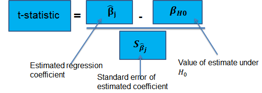
$$ p-value=2\Phi \left( -|{ t }^{ act }| \right) $$

  • Also, the \(t\)-statistic can be compared to the critical value corresponding to the significance level that is desired for the test.

Confidence Intervals for a Single Coefficient

The confidence interval for a regression coefficient in multiple regression is calculated and interpreted the same way as it is in simple linear regression. 

hypothesis test multiple regression

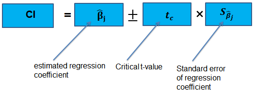
The t-statistic has n – k – 1 degrees of freedom where k = number of independents

Supposing that an interval contains the true value of \({ \beta }_{ j }\) with a probability of 95%. This is simply the 95% two-sided confidence interval for \({ \beta }_{ j }\). The implication here is that the true value of \({ \beta }_{ j }\) is contained in 95% of all possible randomly drawn variables.

Alternatively, the 95% two-sided confidence interval for \({ \beta }_{ j }\) is the set of values that are impossible to reject when a two-sided hypothesis test of 5% is applied. Therefore, with a large sample size:

$$ 95\%\quad confidence\quad interval\quad for\quad { \beta }_{ j }=\left[ { \hat { \beta } }_{ j }-1.96SE\left( { \hat { \beta } }_{ j } \right) ,{ \hat { \beta } }_{ j }+1.96SE\left( { \hat { \beta } }_{ j } \right) \right] $$

Tests of Joint Hypotheses

In this section, we consider the formulation of the joint hypotheses on multiple regression coefficients. We will further study the application of an \(F\)-statistic in their testing.

Hypotheses Testing on Two or More Coefficients

Joint null hypothesis.

In multiple regression, we canno t test the null hypothesis that all slope coefficients are equal 0 based on t -tests that each individual slope coefficient equals 0. Why? individual t-tests do not account for the effects of interactions among the independent variables.

For this reason, we conduct the F-test which uses the F-statistic .  The F-test tests the null hypothesis that all of the slope coefficients in the multiple regression model are jointly equal to 0, .i.e.,

\(F\)-Statistic

The F-statistic, which is always a one-tailed test , is calculated as:

hypothesis test multiple regression

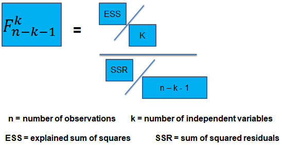
To determine whether at least one of the coefficients is statistically significant, the calculated F-statistic is compared with the one-tailed critical F-value, at the appropriate level of significance.

Decision rule:

hypothesis test multiple regression

Rejection of the null hypothesis at a stated level of significance indicates that at least one of the coefficients is significantly different than zero, i.e, at least one of the independent variables in the regression model makes a significant contribution to the dependent variable.

An analyst runs a regression of monthly value-stock returns on four independent variables over 48 months.

The total sum of squares for the regression is 360, and the sum of squared errors is 120.

Test the null hypothesis at the 5% significance level (95% confidence) that all the four independent variables are equal to zero.

\({ H }_{ 0 }:{ \beta }_{ 1 }=0,{ \beta }_{ 2 }=0,\dots ,{ \beta }_{ 4 }=0 \)

\({ H }_{ 1 }:{ \beta }_{ j }\neq 0\) (at least one j is not equal to zero, j=1,2… k )

ESS = TSS – SSR = 360 – 120 = 240

The calculated test statistic = (ESS/k)/(SSR/(n-k-1))

=(240/4)/(120/43) = 21.5

\({ F }_{ 43 }^{ 4 }\) is approximately 2.44 at 5% significance level.

Decision: Reject H 0 .

Conclusion: at least one of the 4 independents is significantly different than zero.

Omitted Variable Bias in Multiple Regression

This is the bias in the OLS estimator arising when at least one included regressor gets collaborated with an omitted variable. The following conditions must be satisfied for an omitted variable bias to occur:

  • There must be a correlation between at least one of the included regressors and the omitted variable.
  • The dependent variable \(Y\) must be determined by the omitted variable.

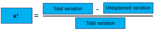
Practical Interpretation of the \({ R }^{ 2 }\) and the adjusted \({ R }^{ 2 }\), \({ \bar { R } }^{ 2 }\)

To determine the accuracy within which the OLS regression line fits the data, we apply the coefficient of determination and the regression’s standard error . 

The coefficient of determination, represented by \({ R }^{ 2 }\), is a measure of the “goodness of fit” of the regression. It is interpreted as the percentage of variation in the dependent variable explained by the independent variables

hypothesis test multiple regression

\({ R }^{ 2 }\) is not a reliable indicator of the explanatory power of a multiple regression model.Why? \({ R }^{ 2 }\) almost always increases as new independent variables are added to the model, even if the marginal contribution of the new variable is not statistically significant. Thus, a high \({ R }^{ 2 }\) may reflect the impact of a large set of independents rather than how well the set explains the dependent.This problem is solved by the use of the adjusted \({ R }^{ 2 }\) (extensively covered in chapter 8)

The following are the factors to watch out when guarding against applying the \({ R }^{ 2 }\) or the \({ \bar { R } }^{ 2 }\):

  • An added variable doesn’t have to be statistically significant just because the \({ R }^{ 2 }\) or the \({ \bar { R } }^{ 2 }\) has increased.
  • It is not always true that the regressors are a true cause of the dependent variable, just because there is a high \({ R }^{ 2 }\) or \({ \bar { R } }^{ 2 }\).
  • It is not necessary that there is no omitted variable bias just because we have a high \({ R }^{ 2 }\) or \({ \bar { R } }^{ 2 }\).
  • It is not necessarily true that we have the most appropriate set of regressors just because we have a high \({ R }^{ 2 }\) or \({ \bar { R } }^{ 2 }\).
  • It is not necessarily true that we have an inappropriate set of regressors just because we have a low \({ R }^{ 2 }\) or \({ \bar { R } }^{ 2 }\).

An economist tests the hypothesis that GDP growth in a certain country can be explained by interest rates and inflation.

Using some 30 observations, the analyst formulates the following regression equation:

$$ GDP growth = { \hat { \beta } }_{ 0 } + { \hat { \beta } }_{ 1 } Interest+ { \hat { \beta } }_{ 2 } Inflation $$

Regression estimates are as follows:


Intercept

0.10

0.5%

Interest rates

0.20

0.05

Inflation

0.15

0.03

Is the coefficient for interest rates significant at 5%?

  • Since the test statistic < t-critical, we accept H 0 ; the interest rate coefficient is  not   significant at the 5% level.
  • Since the test statistic > t-critical, we reject H 0 ; the interest rate coefficient is not significant at the 5% level.
  • Since the test statistic > t-critical, we reject H 0 ; the interest rate coefficient is significant at the 5% level.
  • Since the test statistic < t-critical, we accept H 1 ; the interest rate coefficient is significant at the 5% level.

The correct answer is  C .

We have GDP growth = 0.10 + 0.20(Int) + 0.15(Inf)

Hypothesis:

$$ { H }_{ 0 }:{ \hat { \beta } }_{ 1 } = 0 \quad vs \quad { H }_{ 1 }:{ \hat { \beta } }_{ 1 }≠0 $$

The test statistic is:

$$ t = \left( \frac { 0.20 – 0 }{ 0.05 } \right)  = 4 $$

The critical value is t (α/2, n-k-1) = t 0.025,27  = 2.052 (which can be found on the t-table).

t-table-25-29

Conclusion : The interest rate coefficient is significant at the 5% level.

Offered by AnalystPrep

hypothesis test multiple regression

Modeling Cycles: MA, AR, and ARMA Models

Empirical approaches to risk metrics and hedging, futures markets.

After completing this reading, you should be able to: Define and describe the... Read More

Bond Yields and Return Calculations

After completing this reading, you should be able to: Distinguish between gross, and... Read More

Modeling and Forecasting Seasonality

After completing this reading you should be able to: Describe the sources of... Read More

Modeling and Hedging Non-Parallel Term ...

After completing this reading you should be able to: Describe principal components analysis... Read More

Leave a Comment Cancel reply

You must be logged in to post a comment.

Have a language expert improve your writing

Run a free plagiarism check in 10 minutes, generate accurate citations for free.

  • Knowledge Base

Multiple Linear Regression | A Quick Guide (Examples)

Published on February 20, 2020 by Rebecca Bevans . Revised on June 22, 2023.

Regression models are used to describe relationships between variables by fitting a line to the observed data. Regression allows you to estimate how a dependent variable changes as the independent variable(s) change.

Multiple linear regression is used to estimate the relationship between  two or more independent variables and one dependent variable . You can use multiple linear regression when you want to know:

  • How strong the relationship is between two or more independent variables and one dependent variable (e.g. how rainfall, temperature, and amount of fertilizer added affect crop growth).
  • The value of the dependent variable at a certain value of the independent variables (e.g. the expected yield of a crop at certain levels of rainfall, temperature, and fertilizer addition).

Table of contents

Assumptions of multiple linear regression, how to perform a multiple linear regression, interpreting the results, presenting the results, other interesting articles, frequently asked questions about multiple linear regression.

Multiple linear regression makes all of the same assumptions as simple linear regression :

Homogeneity of variance (homoscedasticity) : the size of the error in our prediction doesn’t change significantly across the values of the independent variable.

Independence of observations : the observations in the dataset were collected using statistically valid sampling methods , and there are no hidden relationships among variables.

In multiple linear regression, it is possible that some of the independent variables are actually correlated with one another, so it is important to check these before developing the regression model. If two independent variables are too highly correlated (r2 > ~0.6), then only one of them should be used in the regression model.

Normality : The data follows a normal distribution .

Linearity : the line of best fit through the data points is a straight line, rather than a curve or some sort of grouping factor.

Receive feedback on language, structure, and formatting

Professional editors proofread and edit your paper by focusing on:

  • Academic style
  • Vague sentences
  • Style consistency

See an example

hypothesis test multiple regression

Multiple linear regression formula

The formula for a multiple linear regression is:

y = {\beta_0} + {\beta_1{X_1}} + … + {{\beta_n{X_n}} + {\epsilon}

  • … = do the same for however many independent variables you are testing

B_nX_n

To find the best-fit line for each independent variable, multiple linear regression calculates three things:

  • The regression coefficients that lead to the smallest overall model error.
  • The t statistic of the overall model.
  • The associated p value (how likely it is that the t statistic would have occurred by chance if the null hypothesis of no relationship between the independent and dependent variables was true).

It then calculates the t statistic and p value for each regression coefficient in the model.

Multiple linear regression in R

While it is possible to do multiple linear regression by hand, it is much more commonly done via statistical software. We are going to use R for our examples because it is free, powerful, and widely available. Download the sample dataset to try it yourself.

Dataset for multiple linear regression (.csv)

Load the heart.data dataset into your R environment and run the following code:

This code takes the data set heart.data and calculates the effect that the independent variables biking and smoking have on the dependent variable heart disease using the equation for the linear model: lm() .

Learn more by following the full step-by-step guide to linear regression in R .

To view the results of the model, you can use the summary() function:

This function takes the most important parameters from the linear model and puts them into a table that looks like this:

R multiple linear regression summary output

The summary first prints out the formula (‘Call’), then the model residuals (‘Residuals’). If the residuals are roughly centered around zero and with similar spread on either side, as these do ( median 0.03, and min and max around -2 and 2) then the model probably fits the assumption of heteroscedasticity.

Next are the regression coefficients of the model (‘Coefficients’). Row 1 of the coefficients table is labeled (Intercept) – this is the y-intercept of the regression equation. It’s helpful to know the estimated intercept in order to plug it into the regression equation and predict values of the dependent variable:

The most important things to note in this output table are the next two tables – the estimates for the independent variables.

The Estimate column is the estimated effect , also called the regression coefficient or r 2 value. The estimates in the table tell us that for every one percent increase in biking to work there is an associated 0.2 percent decrease in heart disease, and that for every one percent increase in smoking there is an associated .17 percent increase in heart disease.

The Std.error column displays the standard error of the estimate. This number shows how much variation there is around the estimates of the regression coefficient.

The t value column displays the test statistic . Unless otherwise specified, the test statistic used in linear regression is the t value from a two-sided t test . The larger the test statistic, the less likely it is that the results occurred by chance.

The Pr( > | t | ) column shows the p value . This shows how likely the calculated t value would have occurred by chance if the null hypothesis of no effect of the parameter were true.

Because these values are so low ( p < 0.001 in both cases), we can reject the null hypothesis and conclude that both biking to work and smoking both likely influence rates of heart disease.

When reporting your results, include the estimated effect (i.e. the regression coefficient), the standard error of the estimate, and the p value. You should also interpret your numbers to make it clear to your readers what the regression coefficient means.

Visualizing the results in a graph

It can also be helpful to include a graph with your results. Multiple linear regression is somewhat more complicated than simple linear regression, because there are more parameters than will fit on a two-dimensional plot.

However, there are ways to display your results that include the effects of multiple independent variables on the dependent variable, even though only one independent variable can actually be plotted on the x-axis.

Multiple regression in R graph

Here, we have calculated the predicted values of the dependent variable (heart disease) across the full range of observed values for the percentage of people biking to work.

To include the effect of smoking on the independent variable, we calculated these predicted values while holding smoking constant at the minimum, mean , and maximum observed rates of smoking.

Here's why students love Scribbr's proofreading services

Discover proofreading & editing

If you want to know more about statistics , methodology , or research bias , make sure to check out some of our other articles with explanations and examples.

  • Chi square test of independence
  • Statistical power
  • Descriptive statistics
  • Degrees of freedom
  • Pearson correlation
  • Null hypothesis

Methodology

  • Double-blind study
  • Case-control study
  • Research ethics
  • Data collection
  • Hypothesis testing
  • Structured interviews

Research bias

  • Hawthorne effect
  • Unconscious bias
  • Recall bias
  • Halo effect
  • Self-serving bias
  • Information bias

A regression model is a statistical model that estimates the relationship between one dependent variable and one or more independent variables using a line (or a plane in the case of two or more independent variables).

A regression model can be used when the dependent variable is quantitative, except in the case of logistic regression, where the dependent variable is binary.

Multiple linear regression is a regression model that estimates the relationship between a quantitative dependent variable and two or more independent variables using a straight line.

Linear regression most often uses mean-square error (MSE) to calculate the error of the model. MSE is calculated by:

  • measuring the distance of the observed y-values from the predicted y-values at each value of x;
  • squaring each of these distances;
  • calculating the mean of each of the squared distances.

Linear regression fits a line to the data by finding the regression coefficient that results in the smallest MSE.

Cite this Scribbr article

If you want to cite this source, you can copy and paste the citation or click the “Cite this Scribbr article” button to automatically add the citation to our free Citation Generator.

Bevans, R. (2023, June 22). Multiple Linear Regression | A Quick Guide (Examples). Scribbr. Retrieved September 25, 2024, from https://www.scribbr.com/statistics/multiple-linear-regression/

Is this article helpful?

Rebecca Bevans

Rebecca Bevans

Other students also liked, simple linear regression | an easy introduction & examples, an introduction to t tests | definitions, formula and examples, types of variables in research & statistics | examples, what is your plagiarism score.

logo

Multiple linear regression

Multiple linear regression #.

Fig. 11 Multiple linear regression #

Errors: \(\varepsilon_i \sim N(0,\sigma^2)\quad \text{i.i.d.}\)

Fit: the estimates \(\hat\beta_0\) and \(\hat\beta_1\) are chosen to minimize the residual sum of squares (RSS):

Matrix notation: with \(\beta=(\beta_0,\dots,\beta_p)\) and \({X}\) our usual data matrix with an extra column of ones on the left to account for the intercept, we can write

Multiple linear regression answers several questions #

Is at least one of the variables \(X_i\) useful for predicting the outcome \(Y\) ?

Which subset of the predictors is most important?

How good is a linear model for these data?

Given a set of predictor values, what is a likely value for \(Y\) , and how accurate is this prediction?

The estimates \(\hat\beta\) #

Our goal again is to minimize the RSS: $ \( \begin{aligned} \text{RSS}(\beta) &= \sum_{i=1}^n (y_i -\hat y_i(\beta))^2 \\ & = \sum_{i=1}^n (y_i - \beta_0- \beta_1 x_{i,1}-\dots-\beta_p x_{i,p})^2 \\ &= \|Y-X\beta\|^2_2 \end{aligned} \) $

One can show that this is minimized by the vector \(\hat\beta\) : $ \(\hat\beta = ({X}^T{X})^{-1}{X}^T{y}.\) $

We usually write \(RSS=RSS(\hat{\beta})\) for the minimized RSS.

Which variables are important? #

Consider the hypothesis: \(H_0:\) the last \(q\) predictors have no relation with \(Y\) .

Based on our model: \(H_0:\beta_{p-q+1}=\beta_{p-q+2}=\dots=\beta_p=0.\)

Let \(\text{RSS}_0\) be the minimized residual sum of squares for the model which excludes these variables.

The \(F\) -statistic is defined by: $ \(F = \frac{(\text{RSS}_0-\text{RSS})/q}{\text{RSS}/(n-p-1)}.\) $

Under the null hypothesis (of our model), this has an \(F\) -distribution.

Example: If \(q=p\) , we test whether any of the variables is important. $ \(\text{RSS}_0 = \sum_{i=1}^n(y_i-\overline y)^2 \) $

A anova: 2 × 6
Res.DfRSSDfSum of SqFPr(>F)
<dbl><dbl><dbl><dbl><dbl><dbl>
49411336.29NA NA NA NA
49211078.78 2257.50765.7178530.003509036

The \(t\) -statistic associated to the \(i\) th predictor is the square root of the \(F\) -statistic for the null hypothesis which sets only \(\beta_i=0\) .

A low \(p\) -value indicates that the predictor is important.

Warning: If there are many predictors, even under the null hypothesis, some of the \(t\) -tests will have low p-values even when the model has no explanatory power.

How many variables are important? #

When we select a subset of the predictors, we have \(2^p\) choices.

A way to simplify the choice is to define a range of models with an increasing number of variables, then select the best.

Forward selection: Starting from a null model, include variables one at a time, minimizing the RSS at each step.

Backward selection: Starting from the full model, eliminate variables one at a time, choosing the one with the largest p-value at each step.

Mixed selection: Starting from some model, include variables one at a time, minimizing the RSS at each step. If the p-value for some variable goes beyond a threshold, eliminate that variable.

Choosing one model in the range produced is a form of tuning . This tuning can invalidate some of our methods like hypothesis tests and confidence intervals…

How good are the predictions? #

The function predict in R outputs predictions and confidence intervals from a linear model:

A matrix: 3 × 3 of type dbl
fitlwrupr
9.409426 8.72269610.09616
14.16309013.70842314.61776
18.91675418.20618919.62732

Prediction intervals reflect uncertainty on \(\hat\beta\) and the irreducible error \(\varepsilon\) as well.

A matrix: 3 × 3 of type dbl
fitlwrupr
9.409426 2.94670915.87214
14.163090 7.72089820.60528
18.91675412.45146125.38205

These functions rely on our linear regression model $ \( Y = X\beta + \epsilon. \) $

Dealing with categorical or qualitative predictors #

For each qualitative predictor, e.g. Region :

Choose a baseline category, e.g. East

For every other category, define a new predictor:

\(X_\text{South}\) is 1 if the person is from the South region and 0 otherwise

\(X_\text{West}\) is 1 if the person is from the West region and 0 otherwise.

The model will be: $ \(Y = \beta_0 + \beta_1 X_1 +\dots +\beta_7 X_7 + \color{Red}{\beta_\text{South}} X_\text{South} + \beta_\text{West} X_\text{West} +\varepsilon.\) $

The parameter \(\color{Red}{\beta_\text{South}}\) is the relative effect on Balance (our \(Y\) ) for being from the South compared to the baseline category (East).

The model fit and predictions are independent of the choice of the baseline category.

However, hypothesis tests derived from these variables are affected by the choice.

Solution: To check whether region is important, use an \(F\) -test for the hypothesis \(\beta_\text{South}=\beta_\text{West}=0\) by dropping Region from the model. This does not depend on the coding.

Note that there are other ways to encode qualitative predictors produce the same fit \(\hat f\) , but the coefficients have different interpretations.

So far, we have:

Defined Multiple Linear Regression

Discussed how to test the importance of variables.

Described one approach to choose a subset of variables.

Explained how to code qualitative variables.

Now, how do we evaluate model fit? Is the linear model any good? What can go wrong?

How good is the fit? #

To assess the fit, we focus on the residuals $ \( e = Y - \hat{Y} \) $

The RSS always decreases as we add more variables.

The residual standard error (RSE) corrects this: $ \(\text{RSE} = \sqrt{\frac{1}{n-p-1}\text{RSS}}.\) $

Fig. 12 Residuals #

Visualizing the residuals can reveal phenomena that are not accounted for by the model; eg. synergies or interactions:

Potential issues in linear regression #

Interactions between predictors

Non-linear relationships

Correlation of error terms

Non-constant variance of error (heteroskedasticity)

High leverage points

Collinearity

Interactions between predictors #

Linear regression has an additive assumption: $ \(\mathtt{sales} = \beta_0 + \beta_1\times\mathtt{tv}+ \beta_2\times\mathtt{radio}+\varepsilon\) $

i.e. An increase of 100 USD dollars in TV ads causes a fixed increase of \(100 \beta_2\) USD in sales on average, regardless of how much you spend on radio ads.

We saw that in Fig 3.5 above. If we visualize the fit and the observed points, we see they are not evenly scattered around the plane. This could be caused by an interaction.

One way to deal with this is to include multiplicative variables in the model:

The interaction variable tv \(\cdot\) radio is high when both tv and radio are high.

R makes it easy to include interaction variables in the model:

Non-linearities #

Fig. 13 A nonlinear fit might be better here. #

Example: Auto dataset.

A scatterplot between a predictor and the response may reveal a non-linear relationship.

Solution: include polynomial terms in the model.

Could use other functions besides polynomials…

Fig. 14 Residuals for Auto data #

In 2 or 3 dimensions, this is easy to visualize. What do we do when we have too many predictors?

Correlation of error terms #

We assumed that the errors for each sample are independent:

What if this breaks down?

The main effect is that this invalidates any assertions about Standard Errors, confidence intervals, and hypothesis tests…

Example : Suppose that by accident, we duplicate the data (we use each sample twice). Then, the standard errors would be artificially smaller by a factor of \(\sqrt{2}\) .

When could this happen in real life:

Time series: Each sample corresponds to a different point in time. The errors for samples that are close in time are correlated.

Spatial data: Each sample corresponds to a different location in space.

Grouped data: Imagine a study on predicting height from weight at birth. If some of the subjects in the study are in the same family, their shared environment could make them deviate from \(f(x)\) in similar ways.

Correlated errors #

Simulations of time series with increasing correlations between \(\varepsilon_i\)

Non-constant variance of error (heteroskedasticity) #

The variance of the error depends on some characteristics of the input features.

To diagnose this, we can plot residuals vs. fitted values:

If the trend in variance is relatively simple, we can transform the response using a logarithm, for example.

Outliers from a model are points with very high errors.

While they may not affect the fit, they might affect our assessment of model quality.

Possible solutions: #

If we believe an outlier is due to an error in data collection, we can remove it.

An outlier might be evidence of a missing predictor, or the need to specify a more complex model.

High leverage points #

Some samples with extreme inputs have an outsized effect on \(\hat \beta\) .

This can be measured with the leverage statistic or self influence :

Studentized residuals #

The residual \(e_i = y_i - \hat y_i\) is an estimate for the noise \(\epsilon_i\) .

The standard error of \(\hat \epsilon_i\) is \(\sigma \sqrt{1-h_{ii}}\) .

A studentized residual is \(\hat \epsilon_i\) divided by its standard error (with appropriate estimate of \(\sigma\) )

When model is correct, it follows a Student-t distribution with \(n-p-2\) degrees of freedom.

Collinearity #

Two predictors are collinear if one explains the other well:

Problem: The coefficients become unidentifiable .

Consider the extreme case of using two identical predictors limit : $ \( \begin{aligned} \mathtt{balance} &= \beta_0 + \beta_1\times\mathtt{limit} + \beta_2\times\mathtt{limit} + \epsilon \\ & = \beta_0 + (\beta_1+100)\times\mathtt{limit} + (\beta_2-100)\times\mathtt{limit} + \epsilon \end{aligned} \) $

For every \((\beta_0,\beta_1,\beta_2)\) the fit at \((\beta_0,\beta_1,\beta_2)\) is just as good as at \((\beta_0,\beta_1+100,\beta_2-100)\) .

If 2 variables are collinear, we can easily diagnose this using their correlation.

A group of \(q\) variables is multilinear if these variables “contain less information” than \(q\) independent variables.

Pairwise correlations may not reveal multilinear variables.

The Variance Inflation Factor (VIF) measures how predictable it is given the other variables, a proxy for how necessary a variable is:

Above, \(R^2_{X_j|X_{-j}}\) is the \(R^2\) statistic for Multiple Linear regression of the predictor \(X_j\) onto the remaining predictors.

Multiple Regression: Estimation and Hypothesis Testing


In this chapter we considered the simplest of the multiple regression models, namely, the three-variable linear regression model—one dependent variable and two explanatory variables. Although in many ways a straightforward extension of the two-variable linear regression model, the three-variable model introduced several new concepts, such as partial regression coefficients, adjusted and unadjusted multiple coefficient of determination, and multicollinearity.

Insofar as estimation of the parameters of the multiple regression coefficients is concerned, we still worked within the framework of the classical linear regression model and used the method of ordinary least squares (OLS). The OLS estimators of multiple regression, like the two-variable model, possess several desirable statistical properties summed up in the Gauss-Markov property of best linear unbiased estimators (BLUE).

With the assumption that the disturbance term follows the normal distribution with zero mean and constant variance σ , we saw that, as in the two-variable case, each estimated coefficient in the multiple regression follows the normal distribution with a mean equal to the true population value and the variances given by the formulas developed in the text. Unfortunately, in practice, σ is not known and has to be estimated. The OLS estimator of this unknown variance is . But if we replace σ by , then, as in the two-variable case, each estimated coefficient of the multiple regression follows the distribution, not the normal distribution.

The knowledge that each multiple regression coefficient follows the distribution with d.f. equal to ( ), where is the number of parameters estimated (including the intercept), means we can use the distribution to test statistical hypotheses about each multiple regression coefficient individually. This can be done on the basis of either the test of significance or the confidence interval based on the distribution. In this respect, the multiple regression model does not differ much from the two-variable model, except that proper allowance must be made for the d.f., which now depend on the number of parameters estimated.

However, when testing the hypothesis that all partial slope coefficients are simultaneously equal to zero, the individual testing referred to earlier is of no help. Here we should use the analysis of variance (ANOVA) technique and the attendant test. Incidentally, testing that all partial slope coefficients are simultaneously equal to zero is the same as testing that the multiple coefficient of determination is equal to zero. Therefore, the test can also be used to test this latter but equivalent hypothesis.

We also discussed the question of when to add a variable or a group of variables to a model, using either the test or the test. In this context we also discussed the method of restricted least squares.

All the concepts introduced in this chapter have been illustrated by numerical examples and by concrete economic applications.


To learn more about the book this website supports, please visit its .
and .
is one of the many fine businesses of .
You must be a registered user to view the in this website.

If you already have a username and password, enter it below. If your textbook came with a card and this is your first visit to this site, you can to register.
Username:
Password:
'); document.write(''); } // -->
( )
.'); } else{ document.write('This form changes settings for this website only.'); } //-->
Send mail as:
'); } else { document.write(' '); } } else { document.write(' '); } // -->
'); } else { document.write(' '); } } else { document.write(' '); } document.write('
TA email: '); } else { document.write(' '); } } else { document.write(' '); } // -->
Other email: '); } else { document.write(' '); } } else { document.write(' '); } // -->
"Floating" navigation? '); } else if (floatNav == 2) { document.write(' '); } else { document.write(' '); } // -->
Drawer speed: '; theseOptions += (glideSpeed == 1) ? ' ' : ' ' ; theseOptions += (glideSpeed == 2) ? ' ' : ' ' ; theseOptions += (glideSpeed == 3) ? ' ' : ' ' ; theseOptions += (glideSpeed == 4) ? ' ' : ' ' ; theseOptions += (glideSpeed == 5) ? ' ' : ' ' ; theseOptions += (glideSpeed == 6) ? ' ' : ' ' ; document.write(theseOptions); // -->
1. (optional) Enter a note here:

2. (optional) Select some text on the page (or do this before you open the "Notes" drawer).
3.Highlighter Color:
4.
Search for:
Search in:
Course-wide Content


Instructor Resources


Course-wide Content


Multiple Hypothesis Testing in R

In the first article of this series , we looked at understanding type I and type II errors in the context of an A/B test, and highlighted the issue of “peeking”. In the second , we illustrated a way to calculate always-valid p-values that were immune to peeking. We will now explore multiple hypothesis testing, or what happens when multiple tests are conducted on the same family of data.

We will set things up as before, with the false positive rate \(\alpha = 0.05\) and false negative rate \(\beta=0.20\) .

To illustrate the concepts in this article, we are going to use the same monte_carlo utility function that we used previously:

We’ll use the monte_carlo utility function to run 1000 experiments, measuring whether the p.value is less than alpha after n_obs observations . If it is, we reject the null hypothesis. We will set the effect size to 0; we know that there is no effect and that the null hypothesis is globally true. In this case, we expect about 50 rejections and about 950 non-rejections, since 50/1000 would represent our expected maximum false positive rate of 5%.

In practice, we don’t usually test the same thing 1000 times; instead, we test it once and state that there is a maximum 5% chance that we have falsely said there was an effect when there wasn’t one 1 .

The Family-Wise Error Rate (FWER)

Now imagine we test two separate statistics using the same source data, with each test constrained by the same \(\alpha\) and \(\beta\) as before. What is the probability that we will detect at least one false positive considering the results of both tests? This is known as the family-wise error rate (FWER 2 3 ), and would apply to the case where a researcher claims there is a difference between the populations if any of the tests yields a positive result. It’s clear that this could present issues, as the family-wise error rate Wikipedia page illustrates:

Suppose the treatment is a new way of teaching writing to students, and the control is the standard way of teaching writing. Students in the two groups can be compared in terms of grammar, spelling, organization, content, and so on. As more attributes are compared, it becomes increasingly likely that the treatment and control groups will appear to differ on at least one attribute due to random sampling error alone.

What is the FWER for the two tests? To calculate the probability that at least one false positive will arise in our two-test example, consider that the probability that one test will not reject the null is \(1-\alpha\) . Thus, the probability that both tests will not reject the null is \((1-\alpha)^2)\) and the probability that at least one test will reject the null is \(1-(1-\alpha)^2\) . For \(m\) tests, this generalizes to \(1-(1-\alpha)^m\) . With \(\alpha=0.05\) and \(m=2\) , we have:

Let’s see if we can produce the same result with a Monte Carlo simulation. We will run the Monte Carlo for n_trials and run n_tests_per_trial . For each trial, if at least one of the n_tests_per_trial results in a rejection of the null, we consider that the trial rejects the null. We should see that about 1 in 10 trials reject the null. This is implemented below:

Both results show that evaluating two tests on the same family of data will lead to a ~10% chance that a researcher will claim a “significant” result if they look for either test to reject the null. Any claim there is a maximum 5% false positive rate would be mistaken. As an exercise, verify that doing the same on \(m=4\) tests will lead to an ~18% chance!

A bad testing platform would be one that claims a maximum 5% false positive rate when any one of multiple tests on the same family of data show significance at the 5% level. Clearly, if a researcher is going to claim that the FWER is no more than \(\alpha\) , then they must control for the FWER and carefully consider how individual tests reject the null.

Controlling the FWER

There are many ways to control for the FWER, and the most conservative is the Bonferroni correction . The “Bonferroni method” will reject null hypotheses if \(p_i \le \frac{\alpha}{m}\) . Let’s switch our reject_at_i function for a p_value_at_i function, and then add in the Bonferroni correction:

With the Bonferroni correction, we see that the realized false positive rate is back near the 5% level. Note that we use any(...) to add 1 if any hypothesis is rejected.

Until now, we have only shown that the Bonferroni correction controls the FWER for the case that all null hypotheses are actually true: the effect is set to zero. This is called controlling in the weak sense . Next, let’s use R’s p.adjust function to illustrate the Bonferroni and Holm adjustments to the p-values:

We see that the Holm correction is very similar to the Bonferroni correction in the case that the null hypothesis is always true.

Strongly controlling the FWER

Both the Bonferroni and Holm corrections guarantee that the FWER is controlled in the strong sense , in which we have any configuration of true and non-true null hypothesis. This is ideal, because in reality, we do not know if there is an effect or not.

The Holm correction is uniformly more powerful than the Bonferroni correction, meaning that in the case that there is an effect and the null is false, using the Holm correction will be more likely to detect positives.

Let’s test this by randomly setting the effect size to the minimum detectable effect in about half the cases. Note the slightly modified p_value_at_i function as well as the null_true variable, which will randomly decide if there is a minimum detectable effect size or not for that particular trial.

Note that in the below example, we will not calculate the FWER using the same any(...) construct from the previous code segments. If we were to do this, we would see that the both corrections have the same FWER and the same power (since the outcome of the trial is then decided by whether at least one of the hypotheses was rejected for the trial). Instead, we will tabulate the result for each of the hypotheses. We should see the same false positive rate 4 , but great power for the Holm method.

Indeed, we observe that while the realized false positive rates of both the Bonferroni and Holm methods are very similar, the Holm method has greater power. These corrections essentially reduce our threshold for each test so that across the family of tests, we produce false positives with a probability of no more than \(\alpha\) . This comes at the expense of a reduction in power from the optimal power ( \(1-\beta\) ).

We have illustrated two methods for deciding what null hypotheses in a family of tests to reject. The Bonferroni method rejects hypotheses at the \(\alpha/m\) level. The Holm method has a more involved algorithm for which hypotheses to reject. The Bonferroni and Holm methods have the property that they do control the FWER at \(\alpha\) , and Holm is uniformly more powerful than Bonferroni.

This raises an interesting question: What if we are not concerned about controlling the probability of detecting at least one false positive, but something else? We might be more interested in controlling the expected proportion of false discoveries amongst all discoveries, known as the false discovery rate. As a quick preview, let’s calculate the false discovery rate for our two cases:

By choosing to control for a metric other than the FWER, we may be able to produce results with power closer to the optimal power ( \(1-\beta\) ). We will look at the false discovery rate and other measures in a future article.

Roland Stevenson is a data scientist and consultant who may be reached on LinkedIn .

And a maximum 20% chance that we said there wasn’t an effect when there was one. ↩

Hochberg, Y.; Tamhane, A. C. (1987). Multiple Comparison Procedures. New York: Wiley. p. 5. ISBN 978-0-471-82222-6 ↩

A sharper Bonferroni procedure for multiple tests of significance ↩

Verify this by inspecting the table_bf and table_holm variables. ↩

You may leave a comment below or discuss the post in the forum community.rstudio.com .

User Preferences

Content preview.

Arcu felis bibendum ut tristique et egestas quis:

  • Ut enim ad minim veniam, quis nostrud exercitation ullamco laboris
  • Duis aute irure dolor in reprehenderit in voluptate
  • Excepteur sint occaecat cupidatat non proident

Keyboard Shortcuts

Lesson 5: multiple linear regression, overview section  .

In this lesson, we make our first (and last?!) major jump in the course. We move from the simple linear regression model with one predictor to the multiple linear regression model with two or more predictors. That is, we use the adjective "simple" to denote that our model has only predictors, and we use the adjective "multiple" to indicate that our model has at least two predictors.

In the multiple regression setting, because of the potentially large number of predictors, it is more efficient to use matrices to define the regression model and the subsequent analyses. This lesson considers some of the more important multiple regression formulas in matrix form. If you're unsure about any of this, it may be a good time to take a look at this Matrix Algebra Review .

The good news!

The good news is that everything you learned about the simple linear regression model extends — with at most minor modifications — to the multiple linear regression model. Think about it — you don't have to forget all of that good stuff you learned! In particular:

  • The models have similar "LINE" assumptions. The only real difference is that whereas in simple linear regression we think of the distribution of errors at a fixed value of the single predictor, with multiple linear regression we have to think of the distribution of errors at a fixed set of values for all the predictors. All of the model-checking procedures we learned earlier are useful in the multiple linear regression framework, although the process becomes more involved since we now have multiple predictors. We'll explore this issue further in Lesson 7 .
  • The use and interpretation of \(R^2\) in the context of multiple linear regression remains the same. However, with multiple linear regression, we can also make use of an "adjusted" \(R^2\) value, which is useful for model-building purposes. We'll explore this measure further in Lesson 10 .
  • With a minor generalization of the degrees of freedom, we use t -tests and t -intervals for the regression slope coefficients to assess whether a predictor is significantly linearly related to the response, after controlling for the effects of all the other predictors in the model.
  • With a minor generalization of the degrees of freedom, we use prediction intervals for predicting an individual response and confidence intervals for estimating the mean response. We'll explore these further in Lesson 7 .
  • Know how to calculate a confidence interval for a single slope parameter in the multiple regression setting.
  • Be able to interpret the coefficients of a multiple regression model.
  • Understand what the scope of the model is in the multiple regression model.
  • Understand the calculation and interpretation of R 2 in a multiple regression setting.
  • Understand the calculation and use of adjusted R 2 in a multiple regression setting.

Lesson 5 Code Files Section  

Below is a zip file that contains all the data sets used in this lesson:

STAT501_Lesson05.zip

  • babybirds.txt
  • bodyfat.txt
  • hospital_infct.txt
  • fev_dat.txt
  • soapsuds.txt
  • stat_females.txt

Stack Exchange Network

Stack Exchange network consists of 183 Q&A communities including Stack Overflow , the largest, most trusted online community for developers to learn, share their knowledge, and build their careers.

Q&A for work

Connect and share knowledge within a single location that is structured and easy to search.

Multiple linear regression for hypothesis testing

I am familiar with using multiple linear regressions to create models of various variables. However, I was curious if regression tests are ever used to do any sort of basic hypothesis testing. If so, what would those scenarios/hypotheses look like?

  • hypothesis-testing
  • multiple-regression

gung - Reinstate Monica's user avatar

  • 1 $\begingroup$ Can you explain further what you mean? It is very common to test whether the slope parameter for a variable is different from zero. I would call that "hypothesis testing". Are you unaware of that, or do you mean something different? What constitutes a scenario for your purposes? $\endgroup$ –  gung - Reinstate Monica Commented Apr 2, 2012 at 13:24
  • $\begingroup$ I am unaware of that. I was also unsure if regression-based analysis is used for any other sort of hypothesis testing (perhaps about the significance of one variable over another, etc). $\endgroup$ –  cryptic_star Commented Apr 2, 2012 at 14:04

2 Answers 2

Here is a simple example. I don't know if you are familiar with R, but hopefully the code is sufficiently self-explanatory.

Now, lets see what this looks like:

We can focus on the "Coefficients" section of the output. Each parameter estimated by the model gets its own row. The actual estimate itself is listed in the first column. The second column lists the Standard Errors of the estimates, that is, an estimate of how much estimates would 'bounce around' from sample to sample, if we were to repeat this process over and over and over again. More specifically, it is an estimate of the standard deviation of the sampling distribution of the estimate. If we divide each parameter estimate by its SE, we get a t-score , which is listed in the third column; this is used for hypothesis testing, specifically to test whether the parameter estimate is 'significantly' different from 0. The last column is the p-value associated with that t-score. It is the probability of finding an estimated value that far or further from 0, if the null hypothesis were true. Note that if the null hypothesis is not true, it is not clear that this value is telling us anything meaningful at all.

If we look back and forth between the Coefficients table and the true data generating process above, we can see a few interesting things. The intercept is estimated to be -1.8 and its SE is 27, whereas the true value is 15. Because the associated p-value is .95, it would not be considered 'significantly different' from 0 (a type II error ), but it is nonetheless within one SE of the true value. There is thus nothing terribly extreme about this estimate from the perspective of the true value and the amount it ought to fluctuate; we simply have insufficient power to differentiate it from 0. The same story holds, more or less, for x1 . Data analysts would typically say that it is not even 'marginally significant' because its p-value is >.10, however, this is another type II error. The estimate for x2 is quite accurate $.21214\approx.2$, and the p-value is 'highly significant', a correct decision. x3 also could not be differentiated from 0, p=.62, another correct decision (x3 does not show up in the true data generating process above). Interestingly, the p-value is greater than that for x1 , but less than that for the intercept, both of which are type II errors. Finally, if we look below the Coefficients table we see the F-value for the model, which is a simultaneous test. This test checks to see if the model as a whole predicts the response variable better than chance alone. Another way to say this, is whether or not all the estimates should be considered unable to be differentiated from 0. The results of this test suggests that at least some of the parameter estimates are not equal to 0, anther correct decision. Since there are 4 tests above, we would have no protection from the problem of multiple comparisons without this. (Bear in mind that because p-values are random variables--whether something is significant would vary from experiment to experiment, if the experiment were re-run--it is possible for these to be inconsistent with each other. This is discussed on CV here: Significance of coefficients in multiple regression: significant t-test vs. non-significant F-statistic , and the opposite situation here: How can a regression be significant yet all predictors be non-significant , & here: F and t statistics in a regression .) Perhaps curiously, there are no type I errors in this example. At any rate, all 5 of the tests discussed in this paragraph are hypothesis tests.

From your comment, I gather you may also wonder about how to determine if one explanatory variable is more important than another. This is a very common question, but is quite tricky. Imagine wanting to predict the potential for success in a sport based on an athlete's height and weight, and wondering which is more important. A common strategy is to look to see which estimated coefficient is larger. However, these estimates are specific to the units that were used: for example, the coefficient for weight will change depending on whether pounds or kilograms are used. In addition, it is not remotely clear how to equate / compare pounds and inches, or kilograms and centimeters. One strategy people employ is to standardize (i.e., turn into z-scores) their data first. Then these dimensions are in common units (viz., standard deviations), and the coefficients are similar to r-scores . Moreover, it is possible to test if one r-score is larger than another . Unfortunately, this does not get you out of the woods; unless the true r is exactly 0, the estimated r is driven in large part by the range of covariate values that are used. (I don't know how easy it will be to recognize, but @whuber's excellent answer here: Is $R^2$ useful or dangerous , illustrates this point; to see it, just think about how $r=\sqrt{r^2}$.) Thus, the best that can ever be said is that variability in one explanatory variable within a specified range is more important to determining the level of the response than variability in another explanatory variable within another specified range.

Community's user avatar

The essential test in regression models is the Full-Reduced test. This is where you are comparing 2 regression models, the Full model has all the terms in it and the Reduced test has a subset of those terms (the Reduced model needs to be nested in the Full model). The test then tests the null hypothesis that the reduced model fits just as well as the full model and any difference is due to chance.

Common printouts from statistical software include an overall F test, this is just the Full-Reduced test where the reduced test is an intercept only model. They also often print a p-value for each individual predictor, this is just a series of Full-Reduced model tests, in each one the reduced model does not include that specific term. There are many ways to use these tests to answer questions of interest. In fact pretty much every test taught in a introductory stats course can be computed using regression models and the Full-Reduced test and the results will be identical in many cases and a very close approximation in the few others.

Greg Snow's user avatar

Your Answer

Sign up or log in, post as a guest.

Required, but never shown

By clicking “Post Your Answer”, you agree to our terms of service and acknowledge you have read our privacy policy .

Not the answer you're looking for? Browse other questions tagged regression hypothesis-testing multiple-regression or ask your own question .

  • Featured on Meta
  • Preventing unauthorized automated access to the network
  • User activation: Learnings and opportunities
  • Join Stack Overflow’s CEO and me for the first Stack IRL Community Event in...

Hot Network Questions

  • How to format units inside math environment?
  • All combinations of ascending/descending digits
  • Fjord Explorer – a Nagareru crossword
  • How can fideism's pursuit of truth through faith be considered a sound epistemology when mutually exclusive religious beliefs are accepted on faith?
  • What is the simplest formula for calculating the circumference of a circle?
  • A military space Saga with a woman who is a brilliant tactician and strategist
  • Why is my Lenovo ThinkPad running Ubuntu using the e1000e Ethernet driver?
  • How similar were the MC6800 and MOS 6502?
  • Geometry Math Problem Part 2
  • Does copying files from one drive to another also copy previously deleted data from the drive one?
  • If Voyager is still an active NASA spacecraft, does it have a flight director? Is that a part time job?
  • Value of ECDH with ECIES
  • Can we solve the Sorites paradox with probability?
  • What main benefits does the Hex spell's ability check disadvantage provide?
  • How to do automated content publishing from CLI in XMCloud
  • In John 8, why did the Jews call themselves "children of Abraham" not "children of Jacob" or something else?
  • What causes, and how to avoid, finger numbness?
  • Do early termination fees hold up in court?
  • Easily unload gravel from pickup truck
  • Purpose of sleeve on sledge hammer handle
  • Has Azerbaijan signed a contract to purchase JF-17s from Pakistan?
  • CH in non-set theoretic foundations
  • Tikz: On straight lines moving balls on a circle inside a regular polygon
  • The most common one (L)

hypothesis test multiple regression

Click through the PLOS taxonomy to find articles in your field.

For more information about PLOS Subject Areas, click here .

Loading metrics

Open Access

Peer-reviewed

Research Article

Can expected error costs justify testing a hypothesis at multiple alpha levels rather than searching for an elusive optimal alpha?

Roles Conceptualization, Formal analysis, Methodology, Software, Writing – original draft, Writing – review & editing

* E-mail: [email protected]

Affiliation Complexity Science, Meraglim Holdings Corporation, Palm Beach Gardens, FL, United States of America

ORCID logo

  • Janet Aisbett

PLOS

  • Published: September 25, 2024
  • https://doi.org/10.1371/journal.pone.0304675
  • Peer Review
  • Reader Comments

Table 1

Simultaneous testing of one hypothesis at multiple alpha levels can be performed within a conventional Neyman-Pearson framework. This is achieved by treating the hypothesis as a family of hypotheses, each member of which explicitly concerns test level as well as effect size. Such testing encourages researchers to think about error rates and strength of evidence in both the statistical design and reporting stages of a study. Here, we show that these multi-alpha level tests can deliver acceptable expected total error costs. We first present formulas for expected error costs from single alpha and multiple alpha level tests, given prior probabilities of effect sizes that have either dichotomous or continuous distributions. Error costs are tied to decisions, with different decisions assumed for each of the potential outcomes in the multi-alpha level case. Expected total costs for tests at single and multiple alpha levels are then compared with optimal costs. This comparison highlights how sensitive optimization is to estimated error costs and to assumptions about prevalence. Testing at multiple default thresholds removes the need to formally identify decisions, or to model costs and prevalence as required in optimization approaches. Although total expected error costs with this approach will not be optimal, our results suggest they may be lower, on average, than when “optimal” test levels are based on mis-specified models.

Citation: Aisbett J (2024) Can expected error costs justify testing a hypothesis at multiple alpha levels rather than searching for an elusive optimal alpha? PLoS ONE 19(9): e0304675. https://doi.org/10.1371/journal.pone.0304675

Editor: Stephan Leitner, University of Klagenfurt, AUSTRIA

Received: November 2, 2023; Accepted: May 15, 2024; Published: September 25, 2024

Copyright: © 2024 Janet Aisbett. This is an open access article distributed under the terms of the Creative Commons Attribution License , which permits unrestricted use, distribution, and reproduction in any medium, provided the original author and source are credited.

Data Availability: All relevant data are within the manuscript and its Supporting Information files.

Funding: The author(s) received no specific funding for this work.

Competing interests: The authors have declared that no competing interests exist.

1. Introduction

A long-standing debate concerns which, if any, alpha levels are appropriate to use as thresholds in statistical hypothesis testing, e.g., [ 1 ]. Among the issues raised is how the costs of errors should affect thresholds [ 2 ]. One approach is to determine optimal alpha levels based on these costs, or on broader decision costs, in a given research context.

When Type II error rates are presented as functions of the alpha level, a level can be selected that minimizes the sum of Type I and Type II error costs, contingent upon parameter settings such as effect and sample sizes. This is a local view of optimization. Optimization can also be interpreted in a global sense, as minimizing the expected total error cost given the prior probability of the hypothesis being true [ 3 , 4 ]. In either case, the total cost may also incorporate payoffs from correct decisions [ 5 , 6 ].

In the global approach, estimates of the prior probability—also called the base rate or prevalence of true hypotheses—may be based on knowledge about the relationships under consideration, on replication rates in similar studies, or on other domain knowledge [ 7 – 9 ]. The prevalence estimate is then assumed to be the probability mass at the hypothesized effect size, with the remaining mass assigned according to the test hypothesis that the researcher hopes to reject—typically the null hypothesis of no effect. This dichotomous model has been extended to continuous distributions of true effect sizes in a research scenario [ 10 , 11 ].

Despite their mathematical and philosophical appeal, optimization strategies have not been widely adopted by researchers when selecting statistical test levels. This is arguably due to the difficulty of scoping, estimating, and justifying the various costs/payoffs [ 3 ], and of even defining a research scenario in which to estimate priors [ 12 ]. Greenland says that costs cannot be estimated without understanding the goals behind the analysis [ 2 ]. In view of the domain knowledge required, he suggests stakeholders other than researchers may be better placed to determine costs.

When studies involve well understood processes, domain knowledge will also guide estimation of prior probabilities of true hypotheses. Mayo & Morey argue, however, that such estimates require identifying a unique reference class, which is impossible, and, if it were possible, the prevalence proportion or probability would be unknowable [ 12 ].

And yet researchers are told they cannot hope to identify optimal alpha levels without good information about the base rate of true hypotheses and the cost of errors ([ 6 ]: S1 File ). Relying on a standard threshold such as 0.05 is also not recommended, given the broad spread in optimal alpha values seen in plausible scenarios. For example, Miller & Ulrich find very small values are optimal when the prevalence of true hypotheses is low and the relative cost of Type I to Type II errors is high, and larger alphas are optimal when the converse holds [ 5 , 6 ].

An alternative approach

We propose that, rather than try to find an optimum level in the face of such difficulties, researchers should simultaneously test at multiple test levels and report results in terms of these. This approach may deliver acceptable error costs without having to grapple with ill-defined notions of costs and research scenarios.

Simultaneous tests at multiple alpha levels lead to logical inconsistencies—when a hypothesis about a parameter value is rejected at one level but not rejected at another level, what can we say about the parameter value? This logical inconsistency can be overcome by extending the parameter space with an independent parameter that acts as a proxy for the test level [ 13 ]. The test hypothesis is extended with a conjecture about the value of the new parameter, so findings must also say something about it. This construction is simply to generate copies of the original hypothesis that can be identified by their proposed test level. The data are therefore extended so that all the added conjectures are rejected at their designated alpha level.

This construction puts testing at multiple alpha levels within the established field of multiple hypothesis testing. It is formalized mathematically in the S1 File , which also gives an example and shows how results from tests at multiple levels should be reported.

The advantage of such testing over simply reporting a raw P-value is that a priori attention must be paid to expected losses and the relative importance of Type I and Type II error rates and hence sample sizes. The advantage over a conventional Neyman-Pearson approach is that, at the study design stage, researchers have to consider more than one test level, and, at the reporting stage, they must tie findings to test levels.

We will refer to tests using this construction as multi-alpha tests . The remainder of the paper does not refer to the extended hypotheses and will speak of the original hypothesis being rejected at one alpha level but not at another. This is shorthand for saying that the extended hypothesis linked to the first alpha level is rejected but the extended hypothesis linked to the second alpha level is not.

Error considerations in multi-alpha testing concern a family of hypotheses, even if the original research design only concerned one hypothesis. The family-wise error rate is the probability of one or more incorrect decisions. Obviously, family-wise error rates in multi-alpha testing are driven by the worst performers, namely Type I errors due to tests at the least stringent levels and Type II errors at the most stringent levels.

Looking at rates is misleading when alpha levels are explicitly reported alongside findings, because the costs of errors may vary with level. Many journals require that P-values be reported, since different values have different evidential meaning [ 14 ] and may lead to different practical outcomes. For example, when two portfolios are found to outperform the S&P 500 with respective P-values of 0.10 and 0.01, an investment web site [ 15 ] advises that “the investor can be much more confident” of the second portfolio and so might invest more in it.

Thus, rather than a statistical test leading to dichotomous decisions, there may be a range of decisions, each associated with different error costs. A small P-value may be interpreted as strong evidence that triggers a decision bringing a large positive payoff when the finding is correct and a large loss when the finding is incorrect as compared with the payoff when no evidence level is reported. Likewise, finding an effect only at a relatively weak level may lower the cost/payoff. As a result, total costs could on average be lower when hypotheses are tested at multiple alpha levels than when a single default such as 0.05 or 0.005 is applied over many studies.

Below, we generalize error cost calculations to scenarios with continuous effect size distributions and to multi-alpha testing. Examples based on the resulting formulas then compare expected total error costs from multi-alpha tests with costs from tests at single alpha levels, including optimal levels. Our findings support previous conclusions about the difficulty of choosing optimal alpha levels and they again illustrate how an alpha level that under some conditions is close to optimal can, with different prevalence and cost assumptions, bring comparatively high costs.

Testing the same hypothesis at two or more alpha levels smooths expected total error costs. The costs will not be optimal but may be lower on average than costs from tests using “optimal” alpha levels determined using inappropriate models.

2. Expected total cost of errors in a research scenario

We review and generalize conventional cost calculations to cover continuous effect size distributions. Then we adapt cost considerations to deal with multi-alpha tests and show that, in important cases, the expected error costs are a weighted sum of the expected costs of the individual tests.

To illustrate the mathematical formulas, and to highlight issues with their application, we draw on studies in which the subjects are overweight pet dogs and the study purpose is to investigate diets designed to promote weight loss. The primary outcome measure is percentage weight loss. Examples of such research are a large international study into high fiber/high protein diets [ 16 ], a comparison of high fiber/high protein with high fiber/low fat diets [ 17 ], and a study into the effects of enriching a diet with fish oil and soy germ meal [ 18 ]. Numerous published studies into nutritional effects on the weight of companion animals provide the basis for a relevant research scenario. Studies are frequently funded by pet food manufacturers that advertise their products as being based on expert scientific knowledge, as is the case with the studies cited above.

Expected total error costs when testing at a single alpha level

Dichotomous scenario..

Given a research scenario, suppose that proportion P of research hypotheses are true (or, for local optimization, set P = 0.5). Suppose “true” and “false” effect sizes are dichotomously distributed, with d the difference between the two values in a particular study. In our example, P is the proportion of dietary interventions on overweight pets that lead to meaningful weight loss and d is the standardized mean difference in weight loss.

hypothesis test multiple regression

The alpha level that minimizes this cost can be estimated by searching over alpha levels and sample sizes, given prevalence P , effect difference d and relative error cost C 0 / C 1 [ 3 ]. If optimization is against error rates rather than costs, this relative cost is fixed at 1.

In our example, a Type I error might lead veterinarians and dog food manufacturers to promote high fiber/low fat diet for weight loss when a high fiber/high protein diet would work as well and possibly have fewer adverse effects. Conversely, a Type II error might mean that a cheap and easily implemented weight loss approach was overlooked, with possibly less effective or more expensive high protein diets being promoted. Understanding the relative costs of these errors obviously requires expert knowledge of canine diet, obesity issues, weight-loss alternatives and so on. The costs also depend on how large an effect the low-fat diet has on canine weight compared with the other diet.

Continuous scenario.

Suppose a histogram could be formed from the true size of effects of interventions targeting weight loss in companion animals. This histogram would approximate the density function that describes the prevalence of effect sizes in the research scenario.

More generally, let p ( e ) describe the prevalence of effect size e in a domain R (typically, an interval). Let E be the subset of effect sizes which satisfy the test hypothesis that the researcher is seeking to reject. R–E is therefore the subset of effects for which the research hypothesis is true. For example, if veterinarians consider a standardized weight loss of more than 0.1 to be practically meaningful, and the researcher wants to show a diet leads to meaningful weight loss, R–E is anything larger than 0.1.

hypothesis test multiple regression

Although the assumption of a continuous prevalence distribution is appealing, estimating the distribution is potentially even more difficult than estimating a prevalence proportion P in the dichotomous modelling. Any prevalence model compiled from relevant published literature will be distorted by publication bias and by the discrepancies between reported and true effect sizes highlighted by the “reproducibility crisis”.

Expected total error costs when testing one hypothesis at multiple alpha levels (multi-alpha testing)

Decisions, costs, and test levels..

Greenland argues that decisions cannot be justified without explicit costs [ 2 ]. We therefore relate decisions to costs and test levels before extending the cost expressions to multi-alpha testing.

Consider a hypothesis, such as that higher fiber diets increase weight loss in overweight dogs or that an intervention to control an invasive plant species is more efficacious than a standard treatment under some specified conditions. Suppose a set of decisions D(m), m = 0, 1, 2, …, k, concerns potential actions to be taken, with D (0) the decision to take no new action.

For instance, decisions might be directly research-related, such as terms used in reporting the study findings or choices of publication vehicle. Or they might concern practical actions, such as the study team encouraging local veterinarians to recommend low fat diets over high protein diets, or the research sponsor publicizing the benefits of switching to low fat diets, or the sponsor manufacturing low fat products and promoting them as better than high protein products.

The decisions are ordered according to their anticipated payoff C 1 ( m ) compared with the decision D (0) to take no new action, given that the intervention has a meaningful effect. Thus, D ( k ) will bring the greatest payoff C 1 ( k ). For example, publication in a more highly ranked journal may improve the researchers’ resumés. In the canine example, the overall health benefit from weight loss in overweight dogs increases with the number of dogs that switch from high protein to low fat diets; thus the research sponsor offering a low fat product as well as advertising the benefits will have greater payoff than the other actions.

However, deciding D ( m ) when the effect is not meaningful brings a cost, call it C 0 ( m ). These costs are assumed to increase with level m so that decision D ( k ) carries the greatest cost if the intervention has no meaningful effect. This cost might include more critical attention if published findings are not supported by later studies. In the canine example, costs include promotional costs, the continuing health costs for overweight dogs which might have otherwise had a more effective high protein diet, and potential impacts on the researchers’ and sponsor’s reputations.

Finally, assume that a decreasing set of alpha levels α m , m = 1, …, k has been identified, such that decision D ( m ) will be made if the test hypothesis is rejected at alpha level α m but not at level α m +1 . That is, only one decision is to be made, and it will be selected according to the most stringent alpha level at which the test hypothesis is rejected. If the test is not rejected at any of the alphas, then the decision is D (0), do nothing.

Thus, the research team and sponsor might decide to encourage local veterinarians to promote low fat diets over high protein ones if the findings of the canine dietary study are statistically significant at alpha level 0.05; to recommend such diets on the sponsor’s website and to veterinarian societies if findings are significant at level 0.01; and to manufacture low fat products and promote switching to them if findings are significant at level 0.001.

One approach to making such choices is provided at the end of this section, and the Discussion section further looks at how such a set of alpha levels might be identified.

Expected total costs of errors.

Suppose P is the prevalence of true hypotheses in a research scenario in which a dichotomous distribution of effects is assumed (or if error costs are considered locally, set P = 0.5).

Eq ( 1 ) is the expected error cost when a test will result either in a decision involving an action, or in doing nothing, with the action taken when the P-value calculated from the data is below α . In the multiple alpha level testing scenario, however, decision D ( m ) is only made when the P-value lies between α m +1 and α m . For example, local veterinarians would only be enlisted by the canine diet researchers if the findings are statistically significant at level 0.05 but are not at level 0.01, since at the higher level a wider campaign would be undertaken involving veterinarian organizations.

hypothesis test multiple regression

When the effect of an intervention is meaningful, but the test hypothesis is not rejected by a test at some alpha level, the error cost depends on the difference between the largest payoff C 1 ( k ) and the payoff brought by what was decided. That is, if the decision is D ( m ), the loss is C 1 ( k )− C 1 ( m ). In our example, if low fat canine diets are more effective that high protein diets yet the decision was to only promote them through local veterinarians, the loss would be due to the benefit difference between that and the wider advertising campaign and offering of products that saw more overweight dogs put on such diets.

hypothesis test multiple regression

Here, Δ C 0 ( m ; e ) is the difference in costs for decisions D ( m ) and D ( m – 1) when the effect size is e ∈ E , and Δ C 1 ( m ; e ) is the difference between payoffs when e ∈ R–E .

Expected error cost of a multi-alpha test as the weighted sum of the costs of the single level tests

In standard single-level test situations within a conventional Neyman-Pearson framework, the potential research outcomes are independent of test level, according to the “all or nothing” nature of findings when a test threshold is applied. These dichotomous outcomes can plausibly be set to D (0) (do nothing if the test hypothesis is not rejected) and D ( k ). Thus, if the canine diet study gets a significant result, the sponsor will go ahead with manufacturing and marketing a product; otherwise, say, the researchers and the sponsor’s product innovation team may be asked to identify factors affecting the result. The Type I and Type II costs for these decisions are C 0 ( k ) and C 1 ( k ) respectively.

Now suppose that the relative cost r of Type II to Type I errors is the same at each test level, so that C 1 ( m ) = rC 0 ( m ) for m = 1, …, k. For example, if both cost types are proportional to the number of dogs switching to a low fat diet on the basis of a study, and decisions made at the different test levels primarily determine this number, then the ratio would be approximately constant.

In such a case, it is straightforward to show (see S2 File ) that the total cost of the multi-alpha test is a weighted average of the costs of the individual tests given in (1). It follows that the multi-alpha test will always be less costly than the worst, and more costly than the best, of the single level tests. It is thus more costly than the optimal single level test. The case with a continuous distribution of true effects is analogous.

The value of the information obtained from a test

What might be said about the relationship between costs at different test levels? Rafi & Greenland [ 19 ] suggest that the information conveyed by a test with P-value p is represented by the surprisal value −log 2 ( p ). The smaller the p , the more informative the test. In a multi-alpha test, the information conveyed on rejecting a test hypothesis at level α m might therefore be proportional to −log 2 ( α m ).

hypothesis test multiple regression

Therefore, when error costs at each test level are proportional to the surprisal value of that level, the total cost of the multi-alpha test is a weighted average of the costs of the component tests. This analysis carries over to the case of a continuous distribution of true effect sizes.

The S2 File has mathematical details. It also shows how the first equality in (8) can be used to set alpha levels if costs are known, or conversely can be used to guide appropriate decisions given pre-set alpha levels.

The surprisal values of test levels 0.05, 0.01 and 0.001 are respectively 4.3, 6.6 and 10.0. The information brought by the test at level 0.01 is therefore 50% more than that of the test at 0.05, and that brought by the stringent test at level 0.001 is 50% larger again. If experts agree that the error costs associated with the hypothetical decisions in our low fat versus high protein canine diet study increase by much more than 50% between levels, the range of test levels would need to be increased.

Note that transforming P-values to information values assumes no prior knowledge. A small P-value for a non-inferiority test contrasting the effectiveness of drug A with drug B would not be “surprising” if drug A had been shown to be superior in many previous trials. Indeed, over a very large sample, a large P-value would be surprising in this case.

3. Applying the expected cost formulations

We compare expected error costs of multi-alpha tests with those from conventional testing in studies investigating whether an effect size is practically meaningful. This offers insights into the cost behavior of multi-alpha tests, as well as illustrating the sensitivity of optimization and the potential pitfalls of using a single default test level. Research scenarios are modelled using both dichotomous and normally distributed true effect sizes, and costs from tests at multiple alpha levels are compared with those from single level tests and tests at optimal levels.

The first subsection uses cost estimates drawn from a simplified example in which Type II error costs vary with effect size and can be much higher than Type I costs. The second subsection investigates a research scenario in which different research teams anticipate different effect sizes, and so conduct trials with different sample sizes. Both true effect sizes and anticipated effect sizes are assumed to be normally distributed, and costs are reported as the total expected costs averaged over all the research teams.

We apply test alpha levels ranging from extremely weak through to strong to highlight how each of the levels can give a lower expected total error cost than the others under some parameter settings. Throughout, a two-group design with equal groups is assumed, where n is the total sample size, M is the boundary between meaningful and non-meaningful effect sizes, and all alpha levels are with respect to one-sided tests. For the multi-alpha tests, error costs are assumed to be proportional to the surprisal value of the component test level. This simplifying assumption implies no prior knowledge about test outcomes.

S3 File further illustrates the sensitivity of cost computations and the smoothing effect that multi-alpha testing has on error rates. It summarizes results from simulations in which cost differences between test levels are randomly assigned but Type I errors are on average more costly. The simulations apply one-sided test levels commonly found in the literature.

Cost comparisons in an example research scenario

Consider a research scenario of clinical trials investigating Molnupiravir as therapy in non-hospitalized patients with mild to moderate symptoms of Covid 19. Suppose the primary outcome is all-cause hospitalization or death by day 29.

Following Ruggeri et al [ 20 ] and Goswami et al [ 21 ], only consider the economic burden when estimating costs. If an ineffective drug is administered, economic costs stem from the direct price of the drug and from its distribution. If a drug that would reduce hospitalizations is not used, the economic costs stem from hospitalizations and deaths that were not avoided; the lower the risk ratio, the more hospitalizations could have been prevented using the drug, and hence the greater the costs of Type II errors.

Given a study of Molnupiravir in a particular population, suppose the true risk of hospitalization or death is r 1 in the untreated group and r 2 in the treatment group. Let I be the risk of getting mild to moderate Covid in the population of interest. If the average cost of administering Molnupiravir to an individual is c T then, over the population, the per capita cost of administering it to those diagnosed with mild to moderate Covid is C 0 = c T I .

hypothesis test multiple regression

The difference can be negative. The drug would therefore only be economical to administer if the absolute risk reduction exceeds c T / c H , which in this simplified example we take to be the definition of practically meaningful.

A Molnupiravir cost-benefit analysis using US data [ 21 ] set the cost of a treatment course with the drug at $707 and the cost of a Covid hospitalization (without ICU) at $40,000, with the risk of hospitalization for the untreated population about 0.092. On these conservative notions of cost, the risk must be reduced by at least 707/40,000 ≈ 0.018 for the drug rollout to be cost-effective. These values are used in the calculations reported below.

Dichotomous distribution of effects in the research scenario

hypothesis test multiple regression

Table 1 reports expected total error costs for various parameter settings calculated from (1) with β ( d , α ) and costs defined as above (dropping the scale factor I which appears in all terms). Single level tests are at the one-sided alphas shown in columns 2–4, and multi-alpha tests are formed from these three levels. Note that group size 1000 gives a prior calculated power of 80% to detect effect size –0.046 if testing against the break-even point M at alpha level 0.05, assuming risk in the untreated group is 0.092.

thumbnail

  • PPT PowerPoint slide
  • PNG larger image
  • TIFF original image

https://doi.org/10.1371/journal.pone.0304675.t001

The table reveals a range of optimal alpha levels, allowing each the selected single test levels to out-perform the others in some setting. The values P = 0.5 and P = 0.1 respectively model the local or “no information on prevalence” case and the pessimistic research scenario [ 8 ]. If the true risk difference is near the break-even point and prevalence is low, Type I errors dominate and small alphas are optimal. For larger risk differences or higher prevalence, larger alphas help limit the more costly Type II errors.

For the multi-alpha tests, costs are assumed to be proportional to the surprisal value of the component test level, as described earlier. Proportionality could result from deciding only to administer Molnupiravir to a proportion of people with Covid symptoms, for example, limiting the roll-out to some locations, where the proportion depends on the test level at which the hypothesis of no effect is to be rejected. Then, as discussed earlier, the total expected cost of the multi-alpha tests is a weighted sum of the total expected costs of the one-sided tests at each level. Because of the wide range of alphas, these weighted averages can be substantially higher than the optimal costs. We will return to this point in the Discussion.

Continuous distribution of effects in the research scenario

Suppose the risk difference between treatment and control groups in the Molnupiravir studies approximately follows a normal distribution, and that in a study the true risk in the untreated group is r 1 .

Given critical value M + s z α and standard deviations s and ss defined as above, the standard normal cumulative probability at ( r 1 – r 2 + M + s z α )/ ss is the expected Type I error rate for effect sizes r 2 – r 1 larger than M and is the expected power for effect sizes smaller than M . This formulation equates to that given by (10) for calculating expected Type II error rates.

Based on these calculations, Table 2 reports expected total error costs for different research scenario distributions. For the multi-alpha tests, costs are again assumed to be proportional to the surprisal value of the test level, so that the total expected cost is a weighted sum of the single level test costs. This table is striking for the very large alphas it shows optimizing expected total error costs. The wide range of alpha levels involved in the multi-alpha tests again lead to costs that can be far from optimal.

thumbnail

https://doi.org/10.1371/journal.pone.0304675.t002

A normal distribution of true effects about –0.02 is an optimistic research scenario, in that interventions have more than 50% chance of being meaningful (i.e., cost effective). A normal distribution about zero with a tight standard deviation of 0.015 represents a pessimistic scenario, with only 12% chance of meaningful intervention. The test level 0.05 is close to optimal in the pessimistic scenario because Type II errors are rare. Costs are also lower for each test level in this scenario compared with the optimistic scenario because of the low probability of costly Type II errors. This is illustrated graphically in the S4 File .

Note that when Type II errors have higher cost, Neymann advises the test direction should be reversed because Type I errors rates are better controlled [ 22 ]. In this example, decisions would then be made according to the rejection level, if any, of the tests of the hypothesis that Molnupiravir treatment was cost-effective.

A research scenario in which different research teams anticipate different standardized effect sizes

Consider a research scenario in which studies collect evidence about whether an intervention is practically meaningful, in the sense of a standardized effect difference exceeding some boundary value M .

In the study design stages, different research teams make different predictions about the effect size. For example, the core literature might support a value such as M + 0.4, say, but each research team may apply other evidence to adjust its prediction. Suppose these predictions approximately follow a distribution with density function p ′( x ).

Given an anticipated effect size, each research team calculates sample sizes to achieve 80% power at a one-sided test level of 0.025, using the standard formula. For simplicity, suppose each team selects equal sized groups and estimates the same error costs. Finally, assume the true standardized effects in the research scenario follow a continuous distribution with density function p ( x ).

Fig 1A illustrates distributions of true and anticipated effect sizes. Fig 1B shows how the research teams’ sample sizes vary as a function of the effect sizes they anticipate. Fig 1C converts Fig 1B into a density function describing the probability that a sample size is selected in the research scenario. The requirement to achieve 80% power means that teams who are pessimistic about the anticipated effect size may need very large samples.

thumbnail

(a) Distributions of true (solid curve) and anticipated (dashed curve) standardized effect sizes, assuming true effects are centered on M. The dotted curve is the sampling distribution of an effect on the boundary of meaningful effects when total sample size is 98. The heavy vertical line is at the critical value for level 0.025 tests on this sample, indicating a high Type II error rate. (b) Sample sizes as function of anticipated effect size, calculated using normal distribution approximations with α = 0.025 and 80% power. (c) Probability distribution of sample sizes in the research scenario given the distribution of anticipated effect sizes shown in (a).

https://doi.org/10.1371/journal.pone.0304675.g001

The differing sample sizes in the studies affect both Type I and Type II error rates, denoted β 0 and β 1 in Eq ( 2 ). These error rates, and hence the expected total error cost ϖ ( p , α ), are functions of the anticipated effect size x . The expected total cost over all studies at a single test level α is then ∫ ϖ ( p , α ) p ′( x ) dx , for ϖ ( p , α ) as defined in Eq ( 2 ). The multi-alpha expected total cost over all studies is similarly obtained by integrating the expression in (7).

Table 3 reports expected total costs averaged over all studies, for different means of the true effect distribution and different ratios of Type I to Type II error costs. The costs for the tests at the more stringent level hardly vary with cost ratio because the Type I error rate is negligible. The higher Type I error rates for the weak level tests cause costs to decrease with smaller cost ratios.

thumbnail

https://doi.org/10.1371/journal.pone.0304675.t003

Averaged expected costs for the multi-alpha test are intermediate between the costs of the single level tests and can thus be seen as smoothing costs compared with testing at either level as a default. However, the optimal test levels can be even more lenient than we saw in Table 2 , making the optimal average expected costs substantially lower than for the other tests reported in Table 3 .

4. Discussion

A single alpha level cannot be appropriate for all test situations. Yet it is difficult to establish the level at which costs will be approximately minimized in any given research context. As Miller & Ulrich noted [ 6 ], and as our examples show, optimization is very sensitive to the proportion of true test hypotheses in the research scenario. Even allowing for perfect knowledge of the various costs and of the nature of the distribution of true effect, very different alpha levels can be close to optimal with different sample sizes and different parameters of the effect size distribution.

The impact of the research scenario is not surprising, given how true effect size distributions weight expected Type I versus Type II error rates and hence weight relative costs. Previous investigations into optimal test levels modelled effect sizes as taking one of two possible values. We followed [ 11 ] in also investigating research scenarios in which effect sizes are continuously distributed.

We accepted the convention that rejection of the test hypothesis leads to stakeholders “acting as if” the alternate hypothesis is true, and hence assumed that costs in single level tests are independent of the test level. In the multi-alpha tests, findings are tied to their test level. The costs of a false rejection were therefore assumed to be lower if tests at more stringent levels were not rejected, since it is not plausible to “act as if” in the same way. We suggested that the costs at each alpha level might be proportional to the surprisal value (also called information content) of a finding with a P-value at that level. Our reasoning was that, with less information, any response would be more muted and therefore Type I costs would be lower. On the other hand, Type II costs would be lowered when the test hypothesis was rejected at some, but not all, the test levels, because a little information is better than none.

Research is needed into how reporting findings against test levels affects their interpretation, and hence affects costs. This is related to how reporting P-values affects decisions, although multi-alpha test reporting goes further, in explicitly stating, for example, that a study did not provide any information about the efficacy of an intervention at level 0.005 but did at level 0.05. The results presented in section 3 and in the S3 File obviously give just a glimpse into how expected total error costs vary with modelling assumptions. Nevertheless, the results suggest costs from testing at multiple alpha levels are smoothed from the extremes of the costs when tests in different research scenarios are made at one fixed alpha level. Testing at an “optimal” level calculated using models based on incorrect assumptions may also lead to larger costs than testing at multiple levels.

Theoretically, multiple test levels could be chosen to optimize expected total costs, using Eq ( 6 ), say, and searching over the multidimensional space formed by sample size and the vector of alpha levels. The problems of estimating unknowables would obviously be worse, given our cost formulations assign different error costs at each of the levels. Aisbett [ 13 ]: Appendix 2 adapts an optimization strategy to the multi-alpha case in part by making simple assumptions about cost behavior. However, we do not recommend trying to optimize error costs across tests at multiple alphas.

How then should the alpha levels be selected? When an alpha that incurs high costs is included in the set of test levels, the multi-alpha test costs are increased. For example, in the low prevalence conditions in Table 1 , the high Type I error rates from testing at 0.25 blows out the difference between the optimal or best performer costs and those of the multi-alpha test.

With this in mind, we suggest three strategies for setting the alpha levels in a multi-alpha test.

The first approach is to calculate optimal alphas for single level tests against a range of cost and prevalence models that are reasonable for the research scenario, and then use the smallest and largest of these alphas. The expected error costs from the multi-alpha tests will smooth out high costs if incorrect models are chosen.

A second strategy appropriate for applied research is to follow the procedure presented, without justification, in section 2. In this, potential decisions/courses of actions are identified, associated costs are estimated in terms of the consequences of incorrect decisions, and then test alpha levels are assigned. We envisage this to be an informal process rather than a search for a mathematically optimal solution. Greenland [ 2 ] recommends that researchers identify potential stakeholders who may have competing interests and hence differing views on costs, as Neyman illustrated with manufacturers and users of a possibly carcinogenic chemical [ 22 ]. Testing at multiple alpha levels selected a priori may allow these differing views to be incorporated at the study design stage. In the reporting stage too, different stakeholders can act differently on the findings according to their perceptions of costs, since findings are tied to test levels and weaker levels are associated with lower costs.

A third approach that avoids estimating error costs is the pragmatic strategy of assigning default values, guided by common practice in the researcher’s disciplinary area. Common practice may also be incorporated in standards such as those of the U.S. Census Bureau which define “weak”, “moderate”, and “strong” evidence categories of findings through the test levels 0.10, 0.05 and 0.01 [ 23 ]. Default alpha levels might also be assigned indirectly using default effect sizes, such as the Cohen’s d values for “small”, “medium” and “large” effects, given the functional relationships between P-values and effect sizes that depend, inter alia, on sample size and estimated variance. This pragmatic approach is open to the criticisms made about default alphas in the single level case, but, again, it smooths out high costs that arise when a default alpha level is far from optimal.

An appealing variation on this approach builds on links between Bayes factors (BFs) and P-values [ 4 ]. BFs measure the relative evidence provided by the data for the test and alternate hypotheses. Formulas relating P-values to BFs have been provided for various tests and assumed priors [ 24 ]. Supporting software computes alpha levels that deliver a nominated BF for a given sample size, subject to the assumptions. Alpha levels in some multi-alpha tests could therefore be set from multiple BF nominations. Intervals on the BF scale are labelled “weak”, “moderate” and “strong” categories of evidence favoring one hypothesis over the other. The boundaries of these intervals are potential default BF nominations. The corresponding alphas are functions of sample size, avoiding Lindley’s Paradox when sample sizes are large.

Whatever levels are chosen, testing at multiple alphas is subject to the qualifications needed for any application of P-values, which only indicate the degree to which data are unusual if a test hypothesis together with all other modelling assumptions are correct. Data from a repeat of a trial may still, with the same assumptions and tests, yield a different conclusion.

Nevertheless, testing at more than one alpha level discourages dichotomous interpretations of findings and encourages researchers to move beyond p < 0.05. We have shown that, rather than raising total error costs, multi-alpha tests can be seen as a compromise, offering adequate rather than optimal performance. Such costs, however, may be lower than those from optimization approaches based on mis-specified models. Empirical studies involving committed practitioners are needed in diverse fields, such as health, ecology and management science, to better understand the relative cost performance and to evaluate practical strategies for setting test levels.

Supporting information

S1 file. testing one hypothesis at multiple alpha levels: theoretical foundation and indicative reporting..

https://doi.org/10.1371/journal.pone.0304675.s001

S2 File. Total cost of the multi-alpha test as a weighted average of the costs of the individual tests.

https://doi.org/10.1371/journal.pone.0304675.s002

S3 File. Averaged results from simulations with random costs.

https://doi.org/10.1371/journal.pone.0304675.s003

S4 File. Illustration of impact of the distribution of effect sizes in the research scenario on Type I and Type II error rates.

https://doi.org/10.1371/journal.pone.0304675.s004

S5 File. R code to produce all Tables and Figures: See github . com/JA090/ErrorCosts .

https://doi.org/10.1371/journal.pone.0304675.s005

  • View Article
  • Google Scholar
  • PubMed/NCBI
  • 15. Beers B. P-value: what it is, how to calculate it, and why it matters. Investopedia. 2023; investopedia.com/terms/p/P-value.asp . [cited 2023 Aug. 11]

IMAGES

  1. Multiple Linear Regression Hypothesis Testing in Matrix Form

    hypothesis test multiple regression

  2. PPT

    hypothesis test multiple regression

  3. PPT

    hypothesis test multiple regression

  4. PPT

    hypothesis test multiple regression

  5. Hypothesis Tests in Multiple Linear Regression, Part 2

    hypothesis test multiple regression

  6. PPT

    hypothesis test multiple regression

VIDEO

  1. Hypothesis Testing in Simple Linear Regression

  2. Multiple regression, hypothesis testing, model deployment

  3. Regression and test of hypothesis

  4. Hypothesis Testing in multiple Regression Model, ANOVA #22

  5. Hypothesis testing: Linear & Multiple Regression in R

  6. Hypothesis Test for Linear Regression

COMMENTS

  1. PDF Lecture 5 Hypothesis Testing in Multiple Linear Regression

    As in simple linear regression, under the null hypothesis t 0 = βˆ j seˆ(βˆ j) ∼ t n−p−1. We reject H 0 if |t 0| > t n−p−1,1−α/2. This is a partial test because βˆ j depends on all of the other predictors x i, i 6= j that are in the model. Thus, this is a test of the contribution of x j given the other predictors in the model.

  2. Hypothesis Tests and Confidence Intervals in Multiple Regression

    Confidence Intervals for a Single Coefficient. The confidence interval for a regression coefficient in multiple regression is calculated and interpreted the same way as it is in simple linear regression. The t-statistic has n - k - 1 degrees of freedom where k = number of independents. Supposing that an interval contains the true value of ...

  3. PDF Hypothesis Testing in the Multiple regression model

    Testing that individual coefficients take a specific value such as zero or some other value is done in exactly the same way as with the simple two variable regression model. Now suppose we wish to test that a number of coefficients or combinations of coefficients take some particular value. In this case we will use the so called "F-test".

  4. Multiple Linear Regression

    Multiple linear regression formula. The formula for a multiple linear regression is: = the predicted value of the dependent variable. = the y-intercept (value of y when all other parameters are set to 0) = the regression coefficient () of the first independent variable () (a.k.a. the effect that increasing the value of the independent variable ...

  5. 5.3

    A population model for a multiple linear regression model that relates a y -variable to p -1 x -variables is written as. y i = β 0 + β 1 x i, 1 + β 2 x i, 2 + … + β p − 1 x i, p − 1 + ϵ i. We assume that the ϵ i have a normal distribution with mean 0 and constant variance σ 2. These are the same assumptions that we used in simple ...

  6. Lesson 5: Multiple Linear Regression (MLR) Model & Evaluation

    a hypothesis test for testing that a subset — more than one, but not all — of the slope parameters are 0. In this lesson, we also learn how to perform each of the above three hypothesis tests. Key Learning Goals for this Lesson: Be able to interpret the coefficients of a multiple regression model. Understand what the scope of the model is ...

  7. 18.1: Multiple linear regression

    You would then proceed to generate the ANOVA table for hypothesis testing. Rcmdr: Models → Hypothesis testing → ANOVA tables. ... Absence of multicollinearity is important assumption of multiple regression. A partial test is to calculate product moment correlations among predictor variables. For example, when we calculate the correlation ...

  8. Multiple Linear Regression. A complete study

    Hypothesis Test for Predictors. One of the fundamental questions that should be answered while running Multiple Linear Regression is, whether or not, at least one of the predictors is useful in predicting the output. We saw that the three predictors TV, radio and newspaper had a different degree of linear relationship with the sales.

  9. Multiple linear regression

    Solution: To check whether region is important, use an \(F\)-test for the hypothesis \(\beta_\text{South}=\beta_\text{West}=0\) by dropping Region from the model. This does not depend on the coding. ... Defined Multiple Linear Regression. Discussed how to test the importance of variables. Described one approach to choose a subset of variables.

  10. 9.5

    There is a statistical test we can use to determine the overall significance of the regression model. The F-test in Multiple Linear Regression test the following hypotheses: \ (H_0\colon \beta_1=...=\beta_k=0\) \ (H_a\colon \text { At least one }\beta_i\text { is not equal to zero}\) The test statistic for this test, denoted \ (F^*\), follows ...

  11. Multiple Regression: Estimation and Hypothesis Testing

    Multiple Regression: Estimation and Hypothesis Testing. In this chapter we considered the simplest of the multiple regression models, namely, the three-variable linear regression model—one dependent variable and two explanatory variables. Although in many ways a straightforward extension of the two-variable linear regression model, the three ...

  12. PDF Multiple Regression

    can use its P-value to test the null hypothesis that the true value of the coefficient is 0. Using the coefficients from this table, we can write the regression model:. ... Second, multiple regression is an extraordinarily versatile calculation, underly-ing many widely used Statistics methods. A sound understanding of the multiple

  13. PDF 12-1 Multiple Linear Regression Models

    12-2 Hypothesis Tests in Multiple Linear Regression R 2 and Adjusted R The coefficient of multiple determination • For the wire bond pull strength data, we find that R2 = SS R /SS T = 5990.7712/6105.9447 = 0.9811. • Thus, the model accounts for about 98% of the variability in the pull strength response.

  14. PDF Lecture 4 Multiple linear regression

    • Multiple regression in matrix notation • Least squares estimation of model parameters • Maximum likelihood estimation of model parameters • Hypothesis testing. 2 Multiple linear regression We are now considering the model y i = ...

  15. PDF 13 Multiple Linear( Regression(

    In contrast, the simple regression slope is called the marginal (or unadjusted) coefficient. The multiple regression model can be written in matrix form. To estimate the parameters b 0, b 1,..., b p using the principle of least squares, form the sum of squared deviations of the observed yj's from the regression line:

  16. 15.5: Hypothesis Tests for Regression Models

    Okay, suppose you've estimated your regression model. The first hypothesis test you might want to try is one in which the null hypothesis that there is no relationship between the predictors and the outcome, ... 4.354 on 97 degrees of freedom Multiple R-squared: 0.8161, Adjusted R-squared: 0.8123 F-statistic: 215.2 on 2 and 97 DF, p-value ...

  17. 12.2.1: Hypothesis Test for Linear Regression

    The hypotheses are: Find the critical value using dfE = n − p − 1 = 13 for a two-tailed test α = 0.05 inverse t-distribution to get the critical values ± 2.160. Draw the sampling distribution and label the critical values, as shown in Figure 12-14. Figure 12-14: Graph of t-distribution with labeled critical values.

  18. 6.4

    For the simple linear regression model, there is only one slope parameter about which one can perform hypothesis tests. For the multiple linear regression model, there are three different hypothesis tests for slopes that one could conduct. They are: Hypothesis test for testing that all of the slope parameters are 0.

  19. Writing hypothesis for linear multiple regression models

    2. I struggle writing hypothesis because I get very much confused by reference groups in the context of regression models. For my example I'm using the mtcars dataset. The predictors are wt (weight), cyl (number of cylinders), and gear (number of gears), and the outcome variable is mpg (miles per gallon). Say all your friends think you should ...

  20. Multiple Hypothesis Testing in R · R Views

    We will now explore multiple hypothesis testing, or what happens when multiple tests are conducted on the same family of data. We will set things up as before, with the false positive rate α= 0.05 α = 0.05 and false negative rate β =0.20 β = 0.20. library (pwr) library (ggplot2) set.seed(1) mde <- 0.1 # minimum detectable effect.

  21. Understanding the Null Hypothesis for Linear Regression

    xi: The value of the predictor variable xi. Multiple linear regression uses the following null and alternative hypotheses: H0: β1 = β2 = … = βk = 0. HA: β1 = β2 = … = βk ≠ 0. The null hypothesis states that all coefficients in the model are equal to zero. In other words, none of the predictor variables have a statistically ...

  22. Lesson 5: Multiple Linear Regression

    Lesson 5: Multiple Linear Regression. Overview. In this lesson, we make our first (and last?!) major jump in the course. We move from the simple linear regression model with one predictor to the multiple linear regression model with two or more predictors. That is, we use the adjective "simple" to denote that our model has only predictors, and ...

  23. 8.7: Overall F-test in multiple linear regression

    This test is called the overall F-test in MLR and is very similar to the F F -test in a reference-coded One-Way ANOVA model. It tests the null hypothesis that involves setting every coefficient except the y y -intercept to 0 (so all the slope coefficients equal 0). We saw this reduced model in the One-Way material when we considered setting all ...

  24. Multiple linear regression for hypothesis testing

    I am familiar with using multiple linear regressions to create models of various variables. However, I was curious if regression tests are ever used to do any sort of basic hypothesis testing. If so, what would those scenarios/hypotheses look like? regression. hypothesis-testing.

  25. Can expected error costs justify testing a hypothesis at multiple alpha

    Whatever levels are chosen, testing at multiple alphas is subject to the qualifications needed for any application of P-values, which only indicate the degree to which data are unusual if a test hypothesis together with all other modelling assumptions are correct. Data from a repeat of a trial may still, with the same assumptions and tests ...