hypothesis test is left tailed

Statistics Made Easy

How to Identify a Left Tailed Test vs. a Right Tailed Test

In statistics, we use hypothesis tests to determine whether some claim about a population parameter is true or not.

Whenever we perform a hypothesis test, we always write a null hypothesis and an alternative hypothesis , which take the following forms:

H 0 (Null Hypothesis): Population parameter = ≤, ≥ some value

H A (Alternative Hypothesis): Population parameter <, >, ≠ some value

There are three different types of hypothesis tests:

• Two-tailed test: The alternative hypothesis contains the “≠” sign
• Left-tailed test: The alternative hypothesis contains the “<” sign
• Right-tailed test: The alternative hypothesis contains the “>” sign

Notice that we only have to look at the sign in the alternative hypothesis to determine the type of hypothesis test.

Left-tailed test: The alternative hypothesis contains the “<” sign   Right-tailed test: The alternative hypothesis contains the “>” sign

The following examples show how to identify left-tailed and right-tailed tests in practice.

Example: Left-Tailed Test

Suppose it’s assumed that the average weight of a certain widget produced at a factory is 20 grams. However, one inspector believes the true average weight is less than 20 grams.

To test this, he weighs a simple random sample of 20 widgets and obtains the following information:

• n = 20 widgets
• x = 19.8 grams
• s = 3.1 grams

He then performs a hypothesis test using the following null and alternative hypotheses:

H 0 (Null Hypothesis): μ ≥ 20 grams

H A (Alternative Hypothesis): μ < 20 grams

The test statistic is calculated as:

• t  = ( x – µ) / (s/√ n )
• t = (19.8-20) / (3.1/√ 20 )

According to the t-Distribution table , the t critical value at α = .05 and n-1 = 19 degrees of freedom is – 1.729 .

Since the test statistic is not less than this value, the inspector fails to reject the null hypothesis. He does not have sufficient evidence to say that the true mean weight of widgets produced at this factory is less than 20 grams.

Example: Right-Tailed Test

Suppose it’s assumed that the average height of a certain species of plant is 10 inches tall. However, one botanist claims the true average height is greater than 10 inches.

To test this claim, she goes out and measures the height of a simple random sample of 15 plants and obtains the following information:

• n = 15 plants
• x = 11.4 inches
• s = 2.5 inches

She then performs a hypothesis test using the following null and alternative hypotheses:

H 0 (Null Hypothesis): μ ≤ 10 inches

H A (Alternative Hypothesis): μ > 10 inches

• t = (11.4-10) / (2.5/√ 15 )

According to the t-Distribution table , the t critical value at α = .05 and n-1 = 14 degrees of freedom is 1.761 .

Since the test statistic is greater than this value, the botanist can reject the null hypothesis. She has sufficient evidence to say that the true mean height for this species of plant is greater than 10 inches.

Additional Resources

How to Read the t-Distribution Table One Sample t-test Calculator Two Sample t-test Calculator

Featured Posts

Hey there. My name is Zach Bobbitt. I have a Masters of Science degree in Applied Statistics and I’ve worked on machine learning algorithms for professional businesses in both healthcare and retail. I’m passionate about statistics, machine learning, and data visualization and I created Statology to be a resource for both students and teachers alike.  My goal with this site is to help you learn statistics through using simple terms, plenty of real-world examples, and helpful illustrations.

2 Replies to “How to Identify a Left Tailed Test vs. a Right Tailed Test”

This was so helpful you are a life saver. Thank you so much

Left-tailed test example, -2.885 is less than -1.729, why you mention -2.885 is “not lesss” …

Leave a Reply Cancel reply

Your email address will not be published. Required fields are marked *

Join the Statology Community

Sign up to receive Statology's exclusive study resource: 100 practice problems with step-by-step solutions. Plus, get our latest insights, tutorials, and data analysis tips straight to your inbox!

By subscribing you accept Statology's Privacy Policy.

How to Identify a Left Tailed Test vs. a Right Tailed Test

In statistics, we use hypothesis tests to determine whether some claim about a population parameter is true or not.

Whenever we perform a hypothesis test, we always write a null hypothesis and an alternative hypothesis , which take the following forms:

H 0 (Null Hypothesis): Population parameter = ≤, ≥ some value

H A (Alternative Hypothesis): Population parameter , ≠ some value

There are three different types of hypothesis tests:

• Two-tailed test: The alternative hypothesis contains the “≠” sign
• Left-tailed test: The alternative hypothesis contains the “
• Right-tailed test: The alternative hypothesis contains the “>” sign

Notice that we only have to look at the sign in the alternative hypothesis to determine the type of hypothesis test.

Left-tailed test: The alternative hypothesis contains the “   Right-tailed test: The alternative hypothesis contains the “>” sign

The following examples show how to identify left-tailed and right-tailed tests in practice.

Example: Left-Tailed Test

Suppose it’s assumed that the average weight of a certain widget produced at a factory is 20 grams. However, one inspector believes the true average weight is less than 20 grams.

To test this, he weighs a simple random sample of 20 widgets and obtains the following information:

• n = 20 widgets
• x = 19.8 grams
• s = 3.1 grams

He then performs a hypothesis test using the following null and alternative hypotheses:

H 0 (Null Hypothesis): μ ≥ 20 grams

H A (Alternative Hypothesis): μ

The test statistic is calculated as:

• t  = ( x – µ) / (s/√ n )
• t = (19.8-20) / (3.1/√ 20 )

According to the t-Distribution table , the t critical value at α = .05 and n-1 = 19 degrees of freedom is – 1.729 .

Since the test statistic is not less than this value, the inspector fails to reject the null hypothesis. He does not have sufficient evidence to say that the true mean weight of widgets produced at this factory is less than 20 grams.

Example: Right-Tailed Test

Suppose it’s assumed that the average height of a certain species of plant is 10 inches tall. However, one botanist claims the true average height is greater than 10 inches.

To test this claim, she goes out and measures the height of a simple random sample of 15 plants and obtains the following information:

• n = 15 plants
• x = 11.4 inches
• s = 2.5 inches

She then performs a hypothesis test using the following null and alternative hypotheses:

H 0 (Null Hypothesis): μ ≤ 10 inches

H A (Alternative Hypothesis): μ > 10 inches

• t = (11.4-10) / (2.5/√ 15 )

According to the t-Distribution table , the t critical value at α = .05 and n-1 = 14 degrees of freedom is 1.761 .

Since the test statistic is greater than this value, the botanist can reject the null hypothesis. She has sufficient evidence to say that the true mean height for this species of plant is greater than 10 inches.

Additional Resources

How to Read the t-Distribution Table One Sample t-test Calculator Two Sample t-test Calculator

Joint Frequency: Definition & Examples

G-test of goodness of fit: definition + example, related posts, how to normalize data between -1 and 1, vba: how to check if string contains another..., how to interpret f-values in a two-way anova, how to create a vector of ones in..., how to determine if a probability distribution is..., what is a symmetric histogram (definition & examples), how to find the mode of a histogram..., how to find quartiles in even and odd..., how to calculate sxy in statistics (with example), how to calculate sxx in statistics (with example).

Statistics Tutorial

Descriptive statistics, inferential statistics, stat reference, statistics - hypothesis testing a mean (left tailed).

A population mean is an average of value a population.

Hypothesis tests are used to check a claim about the size of that population mean.

Hypothesis Testing a Mean

The following steps are used for a hypothesis test:

• Check the conditions
• Define the claims
• Decide the significance level
• Calculate the test statistic

For example:

• Population : Nobel Prize winners
• Category : Age when they received the prize.

And we want to check the claim:

"The average age of Nobel Prize winners when they received the prize is less than 60"

By taking a sample of 30 randomly selected Nobel Prize winners we could find that:

The mean age in the sample (\(\bar{x}\)) is 62.1

The standard deviation of age in the sample (\(s\)) is 13.46

From this sample data we check the claim with the steps below.

1. Checking the Conditions

The conditions for calculating a confidence interval for a proportion are:

• The sample is randomly selected
• The population data is normally distributed
• Sample size is large enough

A moderately large sample size, like 30, is typically large enough.

In the example, the sample size was 30 and it was randomly selected, so the conditions are fulfilled.

Note: Checking if the data is normally distributed can be done with specialized statistical tests.

2. Defining the Claims

We need to define a null hypothesis (\(H_{0}\)) and an alternative hypothesis (\(H_{1}\)) based on the claim we are checking.

The claim was:

In this case, the parameter is the mean age of Nobel Prize winners when they received the prize (\(\mu\)).

The null and alternative hypothesis are then:

Null hypothesis : The average age was 60.

Alternative hypothesis : The average age was less than 60.

Which can be expressed with symbols as:

\(H_{0}\): \(\mu = 60 \)

\(H_{1}\): \(\mu < 60 \)

This is a ' left tailed' test, because the alternative hypothesis claims that the proportion is less than in the null hypothesis.

If the data supports the alternative hypothesis, we reject the null hypothesis and accept the alternative hypothesis.

Advertisement

3. Deciding the Significance Level

The significance level (\(\alpha\)) is the uncertainty we accept when rejecting the null hypothesis in a hypothesis test.

The significance level is a percentage probability of accidentally making the wrong conclusion.

Typical significance levels are:

• \(\alpha = 0.1\) (10%)
• \(\alpha = 0.05\) (5%)
• \(\alpha = 0.01\) (1%)

A lower significance level means that the evidence in the data needs to be stronger to reject the null hypothesis.

There is no "correct" significance level - it only states the uncertainty of the conclusion.

Note: A 5% significance level means that when we reject a null hypothesis:

We expect to reject a true null hypothesis 5 out of 100 times.

4. Calculating the Test Statistic

The test statistic is used to decide the outcome of the hypothesis test.

The test statistic is a standardized value calculated from the sample.

The formula for the test statistic (TS) of a population mean is:

\(\displaystyle \frac{\bar{x} - \mu}{s} \cdot \sqrt{n} \)

\(\bar{x}-\mu\) is the difference between the sample mean (\(\bar{x}\)) and the claimed population mean (\(\mu\)).

\(s\) is the sample standard deviation .

\(n\) is the sample size.

In our example:

The claimed (\(H_{0}\)) population mean (\(\mu\)) was \( 60 \)

The sample mean (\(\bar{x}\)) was \(62.1\)

The sample standard deviation (\(s\)) was \(13.46\)

The sample size (\(n\)) was \(30\)

So the test statistic (TS) is then:

\(\displaystyle \frac{62.1-60}{13.46} \cdot \sqrt{30} = \frac{2.1}{13.46} \cdot \sqrt{30} \approx 0.156 \cdot 5.477 = \underline{0.855}\)

You can also calculate the test statistic using programming language functions:

With Python use the scipy and math libraries to calculate the test statistic.

With R use built-in math and statistics functions to calculate the test statistic.

5. Concluding

There are two main approaches for making the conclusion of a hypothesis test:

• The critical value approach compares the test statistic with the critical value of the significance level.
• The P-value approach compares the P-value of the test statistic and with the significance level.

Note: The two approaches are only different in how they present the conclusion.

The Critical Value Approach

For the critical value approach we need to find the critical value (CV) of the significance level (\(\alpha\)).

For a population mean test, the critical value (CV) is a T-value from a student's t-distribution .

This critical T-value (CV) defines the rejection region for the test.

The rejection region is an area of probability in the tails of the standard normal distribution.

Because the claim is that the population mean is less than 60, the rejection region is in the left tail:

The student's t-distribution is adjusted for the uncertainty from smaller samples.

This adjustment is called degrees of freedom (df), which is the sample size \((n) - 1\)

In this case the degrees of freedom (df) is: \(30 - 1 = \underline{29} \)

Choosing a significance level (\(\alpha\)) of 0.05, or 5%, we can find the critical T-value from a T-table , or with a programming language function:

With Python use the Scipy Stats library t.ppf() function find the T-Value for an \(\alpha\) = 0.05 at 29 degrees of freedom (df).

With R use the built-in qt() function to find the t-value for an \(\alpha\) = 0.05 at 29 degrees of freedom (df).

Using either method we can find that the critical T-Value is \(\approx \underline{-1.699}\)

For a left tailed test we need to check if the test statistic (TS) is smaller than the critical value (CV).

If the test statistic is smaller the critical value, the test statistic is in the rejection region .

When the test statistic is in the rejection region, we reject the null hypothesis (\(H_{0}\)).

Here, the test statistic (TS) was \(\approx \underline{0.855}\) and the critical value was \(\approx \underline{-1.699}\)

Here is an illustration of this test in a graph:

Since the test statistic was bigger than the critical value we keep the null hypothesis.

This means that the sample data does not support the alternative hypothesis.

And we can summarize the conclusion stating:

The sample data does not support the claim that "The average age of Nobel Prize winners when they received the prize is less than 60" at a 5% significance level .

The P-Value Approach

For the P-value approach we need to find the P-value of the test statistic (TS).

If the P-value is smaller than the significance level (\(\alpha\)), we reject the null hypothesis (\(H_{0}\)).

The test statistic was found to be \( \approx \underline{0.855} \)

For a population proportion test, the test statistic is a T-Value from a student's t-distribution .

Because this is a left tailed test, we need to find the P-value of a t-value smaller than 0.855.

The student's t-distribution is adjusted according to degrees of freedom (df), which is the sample size \((30) - 1 = \underline{29}\)

We can find the P-value using a T-table , or with a programming language function:

With Python use the Scipy Stats library t.cdf() function find the P-value of a T-value smaller than 0.855 at 29 degrees of freedom (df):

With R use the built-in pt() function find the P-value of a T-Value smaller than 0.855 at 29 degrees of freedom (df):

Using either method we can find that the P-value is \(\approx \underline{0.800}\)

This tells us that the significance level (\(\alpha\)) would need to be smaller 0.80, or 80%, to reject the null hypothesis.

This P-value is far bigger than any of the common significance levels (10%, 5%, 1%).

So the null hypothesis is kept at all of these significance levels.

The sample data does not support the claim that "The average age of Nobel Prize winners when they received the prize is less than 60" at a 10%, 5%, or 1% significance level .

Calculating a P-Value for a Hypothesis Test with Programming

Many programming languages can calculate the P-value to decide outcome of a hypothesis test.

Using software and programming to calculate statistics is more common for bigger sets of data, as calculating manually becomes difficult.

The P-value calculated here will tell us the lowest possible significance level where the null-hypothesis can be rejected.

With Python use the scipy and math libraries to calculate the P-value for a left tailed hypothesis test for a mean.

Here, the sample size is 30, the sample mean is 62.1, the sample standard deviation is 13.46, and the test is for a mean smaller 60.

With R use built-in math and statistics functions find the P-value for a left tailed hypothesis test for a mean.

Left-Tailed and Two-Tailed Tests

This was an example of a left tailed test, where the alternative hypothesis claimed that parameter is smaller than the null hypothesis claim.

You can check out an equivalent step-by-step guide for other types here:

• Right-Tailed Test
• Two-Tailed Test

COLOR PICKER

Contact Sales

If you want to use W3Schools services as an educational institution, team or enterprise, send us an e-mail: [email protected]

Report Error

If you want to report an error, or if you want to make a suggestion, send us an e-mail: [email protected]

Top Tutorials

Top references, top examples, get certified.

If you're seeing this message, it means we're having trouble loading external resources on our website.

If you're behind a web filter, please make sure that the domains *.kastatic.org and *.kasandbox.org are unblocked.

To log in and use all the features of Khan Academy, please enable JavaScript in your browser.

Statistics and probability

Course: statistics and probability   >   unit 12.

• Hypothesis testing and p-values

One-tailed and two-tailed tests

• Z-statistics vs. T-statistics
• Small sample hypothesis test
• Large sample proportion hypothesis testing

Want to join the conversation?

• Upvote Button navigates to signup page
• Downvote Button navigates to signup page
• Flag Button navigates to signup page

Video transcript

Six Sigma Study Guide

Study notes and guides for Six Sigma certification tests

Tailed Hypothesis Tests

Posted by Ted Hessing

A tailed hypothesis tests is an assumption about a population parameter. The assumption may or may not be true.  Hypothesis testing is a key procedure in inferential statistics used to make statistical decisions using experimental data.  It is basically an assumption that we make about the population parameter.

Null and alternative hypothesis

Null hypothesis (H 0 ): A statistical hypothesis assumes that the observation is due to the chance factor. In other words, the null hypothesis states that there is no (statistical significance) difference or effect.

Alternative hypothesis (H 1 ): The complementary hypothesis of the null hypothesis is an alternative hypothesis. In other words, the alternative hypothesis shows that observations are the results of a real effect.

What are the tails in a hypothesis test?

A tail in hypothesis testing refers to the tail at either end of a distribution curve. Generally, in hypothesis tests, test statistic means to obtain all of the sample data and convert it to a single value. For example, Z-test calculates Z statistics, t-test calculates t-test statistic, and F-test calculates F values etc., are the test statistics. Test statistics need to compare to an appropriate critical value. A decision can then be made to reject or not reject the null hypothesis.

In probability distribution plots, the shaded area in the plot (one side in one-tailed hypothesis and two sides in a two-tailed hypothesis) indicates the probability of a value falls within that range.

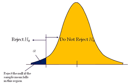
Critical region: In a hypothesis test, critical regions are ranges of the distributions where the values represent statistically significant results. If the test statistic falls in the critical region, reject the null hypothesis.

Types of tailed hypothesis tests

There are three basic types of ‘tails’ that hypothesis tests can have:

• Right-tailed test: where the alternative hypothesis includes a ‘>’ symbol.
• Left-tailed test: where the alternative hypothesis includes a ‘<’ symbol.
• Two-tailed test: where the alternative hypothesis includes a ≠.

One-tailed hypothesis tests

A test of hypothesis where the area of rejection is only in one direction. In other words, when change is expected to have occurred in one direction, i.e expecting output either increase or to decrease.

If the level of significance is 0.05, a one-tail test allots the entire alpha (α) in the one direction to test the statistical significance. Since the statistical significance in the one direction of interest, it is also known as a directional hypothesis.

Reject the null hypothesis; If the test statistic falls in the critical region, that means the test statistic has a greater value than the critical value (for the right-tailed test) and the test statistic has a lesser value than the critical value (for the left tailed test).

Generally, one-tailed tests are more powerful than two-tailed tests; because of that, one-tailed tests are preferred.

The basic disadvantage of a one-tailed test is it considers effects in one direction only. There is a chance that an important effect may miss in another direction. For example, a new material used in the production and checking whether the yield improved over the existing material. There is a possibility that new material may give less yield than the current material.

One tailed tests are further divided into

Right-tailed test

Left-tailed test.

Right tailed test is also called the upper tail test. A hypothesis test is performed if the population parameter is suspected to be greater than the assumed parameter of the null hypothesis.

• H 0 : The sampling mean (x̅) is less than are equal to µ
• H 1 : The sampling mean (x̅) is greater than µ.

Example: The average weight of an iron bar population is 90lbs. Supervisor believes that the average weight might be higher. Random samples of 5 iron bars are measured, and the average weight is 110lbs and a standard deviation of 18lbs. With a 95% confidence level, is there enough evidence to suggest the average weight is higher?

Population average score (µ) = 90

• Sample average (x̅) = 110
• number of samples (n) = 5
• Level of significance α=0.05

H 0 : The average weight is equal to 90, µ=90.

H 1 : The average score is higher than 90, µ>90

Since supervisor is keen to check the average weight is higher, it is a right-tailed test.

Compute the critical value: For 95% confidence level t value with a degrees of freedom n-1= 2.132

Critical value =2.132

Calculate the test statistics t = x̅-µ/(s/√n) = 110-90/(18/√5)=2.484.

Conclusion: Test statistic is greater than the critical value, and it is in the rejection region. Hence, we can reject the null hypothesis. So the average weight of the iron bar is may be higher than the 90lbs.

Left-tailed test is also known as a lower tail test. A hypothesis test is performed if the population parameter is suspected to be less than the assumed parameter of the null hypothesis.

• H 0 : The sampling mean (x̅) is greater than are equal to µ
• H 1 : The sampling mean (x̅) is less than µ.

Example: The average weight of an iron bar population is 90lbs. Supervisor believes that the average weight might be lower. Random samples of 6 iron bars are measured, and the average weight is 82lbs and a standard deviation of 18lbs. With a 95% confidence level, is there enough evidence to suggest the average weight is lower?

• Sample average (x̅) = 82
• number of samples (n) = 6

H 1 : The average score is less than 90, µ<90

Since the supervisor is keen to check the average weight is lower, hence it is a left-tailed test.

Compute the critical value: For 95% confidence level t value with a degrees of freedom n-1= -2.015

Critical value =-2.015

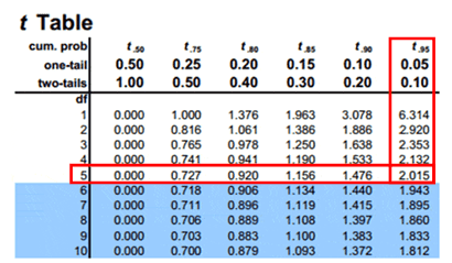
Calculate the test statistics t = x̅-µ/(s/√n) = 82-90/(18/√6)=-1.088

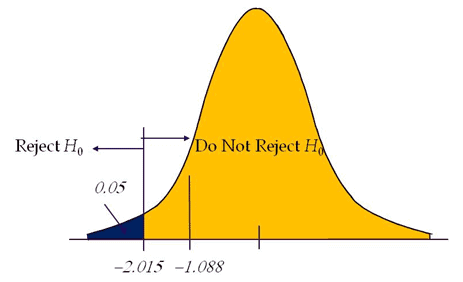
Conclusion: Test statistic is not in the rejection region. Hence, we failed to reject the null hypothesis. So the average weight of the iron bar is 90lbs.

Two-tailed hypothesis tests

A test of hypothesis where the area of rejection is on both sides of the sampling distribution.

If level of significance is 0.05 of a two-tailed test, it distributes the alpha (α) into two equal parts (α/2 & α/2) on both sides to test the statistical significance. 

• H 0 : The sampling mean (x̅) is equal to µ
• H 1 : The sampling mean (x̅) is not equal to µ

Two-tailed tests also known as two-sided or non-directional test, as it tests the effects on both sides. In a two-tailed test, extreme values above or below are evidence against the null hypothesis.

Reject the null hypothesis if test statistics fall on either side of the critical region.

Example: The average score for the mean population is 80, with a standard deviation of 10. With a new training method, the professor believes that the score might change. Professor tested randomly 36 students’ scores. The average score of the sample is 88. With a 95% confidence level, is there enough evidence to suggest the average score changed?

Population average score (µ) = 80

• Sample average (x̅) = 88
• number of samples (n) = 36

H 0 : The average score is equal to 80, µ=80.

H 1 : The average score is not equal to 80, µ≠80

Since the professor is keen to check the change in average score, it is a two tail test

Compute the critical value: For 95% confidence level Z value = 1.96

Critical value =±1.96

Calculate the test statistics Z = x̅-µ/(σ/√n) = 88-80/(10/√36)=4.8

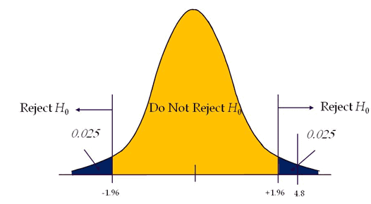
Conclusion: The test statistic is greater than the critical value, which means the test statistic is in the rejection region. So, we can reject the null hypothesis.

Few more Example

For Example, consider a null hypothesis that states that cars traveling on a particular road have a mean velocity of 40 miles/hour:

• A right-tailed test would state that cars traveling on a particular road have a mean velocity greater than 40 miles/hour.
• A left-tailed test would state that cars traveling on a particular road have a mean velocity less than 40 miles/hour.
• A two-tailed test would state that cars traveling on a particular road have a mean velocity greater than or less than 40 miles/hour.

Additional Resources:

• https://www.statisticshowto.datasciencecentral.com/how-to-decide-if-a-hypothesis-test-is-a-left-tailed-test-or-a-right-tailed-test/  

Important Videos

I originally created SixSigmaStudyGuide.com to help me prepare for my own Black belt exams. Overtime I've grown the site to help tens of thousands of Six Sigma belt candidates prepare for their Green Belt & Black Belt exams. Go here to learn how to pass your Six Sigma exam the 1st time through!

Comments (8)

I believe you have the right tail and left tails mixed up in this article. It conflicts with other articles you have written and also with my separate findings. In general, the right tailed test is when the alternative hypothesis is > null hypothesis. Putting you on the right side of the bell curve, hence the “right tailed” name.

You’re absolutely correct, Montgomery. The article has been updated. Thanks for bringing this to my attention!

Good Day Ted,

Just brushing up a little while on my break at work. Has the following below been updated yet? When looking at an actual graph it’s otherwise.

-When performing a right-tailed test, we reject the null hypothesis if the test statistics are less than the critical value.

-When performing a left-tailed test, we reject the null hypothesis if the test statistics are greater than the critical value.

We should be all set now with our current re-write, Lemarcus.

Thank you for the note!

What is the difference btw z statistic and t statistic ?

I have seen on your content that, for a right tailed test

For Z statistic, reject null hypothesis if p value is less than critical value

For t statistic, reject null hypothesis if t value is more than critical value

Also, in the two-tailed test, you chose Z instead of t statistic. Why ?

Hello Rahul,

A t-test is used to compare the mean of two given samples. Like a z-test, a t-test also assumes a normal distribution of the sample. A t-test is used when the population parameters (mean and standard deviation) are not known.

Since we know the population mean and standard deviation, selected the z test instead of t test

Your explanations are better and easier to follow than those of my Statistics profs… Thanks

Thanks, Ben. That’s high praise!

Leave a Reply Cancel reply

Your email address will not be published. Required fields are marked *

This site uses Akismet to reduce spam. Learn how your comment data is processed .

Insert/edit link

Enter the destination URL

Or link to existing content

User Preferences

Content preview.

Arcu felis bibendum ut tristique et egestas quis:

• Ut enim ad minim veniam, quis nostrud exercitation ullamco laboris
• Duis aute irure dolor in reprehenderit in voluptate
• Excepteur sint occaecat cupidatat non proident

Keyboard Shortcuts

S.3.1 hypothesis testing (critical value approach).

The critical value approach involves determining "likely" or "unlikely" by determining whether or not the observed test statistic is more extreme than would be expected if the null hypothesis were true. That is, it entails comparing the observed test statistic to some cutoff value, called the " critical value ." If the test statistic is more extreme than the critical value, then the null hypothesis is rejected in favor of the alternative hypothesis. If the test statistic is not as extreme as the critical value, then the null hypothesis is not rejected.

Specifically, the four steps involved in using the critical value approach to conducting any hypothesis test are:

• Specify the null and alternative hypotheses.
• Using the sample data and assuming the null hypothesis is true, calculate the value of the test statistic. To conduct the hypothesis test for the population mean μ , we use the t -statistic \(t^*=\frac{\bar{x}-\mu}{s/\sqrt{n}}\) which follows a t -distribution with n - 1 degrees of freedom.
• Determine the critical value by finding the value of the known distribution of the test statistic such that the probability of making a Type I error — which is denoted \(\alpha\) (greek letter "alpha") and is called the " significance level of the test " — is small (typically 0.01, 0.05, or 0.10).
• Compare the test statistic to the critical value. If the test statistic is more extreme in the direction of the alternative than the critical value, reject the null hypothesis in favor of the alternative hypothesis. If the test statistic is less extreme than the critical value, do not reject the null hypothesis.

Example S.3.1.1

Mean gpa section  .

In our example concerning the mean grade point average, suppose we take a random sample of n = 15 students majoring in mathematics. Since n = 15, our test statistic t * has n - 1 = 14 degrees of freedom. Also, suppose we set our significance level α at 0.05 so that we have only a 5% chance of making a Type I error.

Right-Tailed

The critical value for conducting the right-tailed test H 0 : μ = 3 versus H A : μ > 3 is the t -value, denoted t \(\alpha\) , n - 1 , such that the probability to the right of it is \(\alpha\). It can be shown using either statistical software or a t -table that the critical value t 0.05,14 is 1.7613. That is, we would reject the null hypothesis H 0 : μ = 3 in favor of the alternative hypothesis H A : μ > 3 if the test statistic t * is greater than 1.7613. Visually, the rejection region is shaded red in the graph.

Left-Tailed

The critical value for conducting the left-tailed test H 0 : μ = 3 versus H A : μ < 3 is the t -value, denoted -t ( \(\alpha\) , n - 1) , such that the probability to the left of it is \(\alpha\). It can be shown using either statistical software or a t -table that the critical value -t 0.05,14 is -1.7613. That is, we would reject the null hypothesis H 0 : μ = 3 in favor of the alternative hypothesis H A : μ < 3 if the test statistic t * is less than -1.7613. Visually, the rejection region is shaded red in the graph.

There are two critical values for the two-tailed test H 0 : μ = 3 versus H A : μ ≠ 3 — one for the left-tail denoted -t ( \(\alpha\) / 2, n - 1) and one for the right-tail denoted t ( \(\alpha\) / 2, n - 1) . The value - t ( \(\alpha\) /2, n - 1) is the t -value such that the probability to the left of it is \(\alpha\)/2, and the value t ( \(\alpha\) /2, n - 1) is the t -value such that the probability to the right of it is \(\alpha\)/2. It can be shown using either statistical software or a t -table that the critical value -t 0.025,14 is -2.1448 and the critical value t 0.025,14 is 2.1448. That is, we would reject the null hypothesis H 0 : μ = 3 in favor of the alternative hypothesis H A : μ ≠ 3 if the test statistic t * is less than -2.1448 or greater than 2.1448. Visually, the rejection region is shaded red in the graph.

Critical Value Calculator

How to use critical value calculator, what is a critical value, critical value definition, how to calculate critical values, z critical values, t critical values, chi-square critical values (χ²), f critical values, behind the scenes of the critical value calculator.

Welcome to the critical value calculator! Here you can quickly determine the critical value(s) for two-tailed tests, as well as for one-tailed tests. It works for most common distributions in statistical testing: the standard normal distribution N(0,1) (that is when you have a Z-score), t-Student, chi-square, and F-distribution .

What is a critical value? And what is the critical value formula? Scroll down – we provide you with the critical value definition and explain how to calculate critical values in order to use them to construct rejection regions (also known as critical regions).

The critical value calculator is your go-to tool for swiftly determining critical values in statistical tests, be it one-tailed or two-tailed. To effectively use the calculator, follow these steps:

In the first field, input the distribution of your test statistic under the null hypothesis: is it a standard normal N (0,1), t-Student, chi-squared, or Snedecor's F? If you are not sure, check the sections below devoted to those distributions, and try to localize the test you need to perform.

In the field What type of test? choose the alternative hypothesis : two-tailed, right-tailed, or left-tailed.

If needed, specify the degrees of freedom of the test statistic's distribution. If you need more clarification, check the description of the test you are performing. You can learn more about the meaning of this quantity in statistics from the degrees of freedom calculator .

Set the significance level, α \alpha α . By default, we pre-set it to the most common value, 0.05, but you can adjust it to your needs.

The critical value calculator will display your critical value(s) and the rejection region(s).

Click the advanced mode if you need to increase the precision with which the critical values are computed.

For example, let's envision a scenario where you are conducting a one-tailed hypothesis test using a t-Student distribution with 15 degrees of freedom. You have opted for a right-tailed test and set a significance level (α) of 0.05. The results indicate that the critical value is 1.7531, and the critical region is (1.7531, ∞). This implies that if your test statistic exceeds 1.7531, you will reject the null hypothesis at the 0.05 significance level.

👩‍🏫 Want to learn more about critical values? Keep reading!

In hypothesis testing, critical values are one of the two approaches which allow you to decide whether to retain or reject the null hypothesis. The other approach is to calculate the p-value (for example, using the p-value calculator ).

The critical value approach consists of checking if the value of the test statistic generated by your sample belongs to the so-called rejection region , or critical region , which is the region where the test statistic is highly improbable to lie . A critical value is a cut-off value (or two cut-off values in the case of a two-tailed test) that constitutes the boundary of the rejection region(s). In other words, critical values divide the scale of your test statistic into the rejection region and the non-rejection region.

Once you have found the rejection region, check if the value of the test statistic generated by your sample belongs to it :

• If so, it means that you can reject the null hypothesis and accept the alternative hypothesis; and
• If not, then there is not enough evidence to reject H 0 .

But how to calculate critical values? First of all, you need to set a significance level , α \alpha α , which quantifies the probability of rejecting the null hypothesis when it is actually correct. The choice of α is arbitrary; in practice, we most often use a value of 0.05 or 0.01. Critical values also depend on the alternative hypothesis you choose for your test , elucidated in the next section .

To determine critical values, you need to know the distribution of your test statistic under the assumption that the null hypothesis holds. Critical values are then points with the property that the probability of your test statistic assuming values at least as extreme at those critical values is equal to the significance level α . Wow, quite a definition, isn't it? Don't worry, we'll explain what it all means.

First, let us point out it is the alternative hypothesis that determines what "extreme" means. In particular, if the test is one-sided, then there will be just one critical value; if it is two-sided, then there will be two of them: one to the left and the other to the right of the median value of the distribution.

Critical values can be conveniently depicted as the points with the property that the area under the density curve of the test statistic from those points to the tails is equal to α \alpha α :

Left-tailed test: the area under the density curve from the critical value to the left is equal to α \alpha α ;

Right-tailed test: the area under the density curve from the critical value to the right is equal to α \alpha α ; and

Two-tailed test: the area under the density curve from the left critical value to the left is equal to α / 2 \alpha/2 α /2 , and the area under the curve from the right critical value to the right is equal to α / 2 \alpha/2 α /2 as well; thus, total area equals α \alpha α .

As you can see, finding the critical values for a two-tailed test with significance α \alpha α boils down to finding both one-tailed critical values with a significance level of α / 2 \alpha/2 α /2 .

The formulae for the critical values involve the quantile function , Q Q Q , which is the inverse of the cumulative distribution function ( c d f \mathrm{cdf} cdf ) for the test statistic distribution (calculated under the assumption that H 0 holds!): Q = c d f − 1 Q = \mathrm{cdf}^{-1} Q = cdf − 1 .

Once we have agreed upon the value of α \alpha α , the critical value formulae are the following:

• Left-tailed test :
• Right-tailed test :
• Two-tailed test :

In the case of a distribution symmetric about 0 , the critical values for the two-tailed test are symmetric as well:

Unfortunately, the probability distributions that are the most widespread in hypothesis testing have somewhat complicated c d f \mathrm{cdf} cdf formulae. To find critical values by hand, you would need to use specialized software or statistical tables. In these cases, the best option is, of course, our critical value calculator! 😁

Use the Z (standard normal) option if your test statistic follows (at least approximately) the standard normal distribution N(0,1) .

In the formulae below, u u u denotes the quantile function of the standard normal distribution N(0,1):

Left-tailed Z critical value: u ( α ) u(\alpha) u ( α )

Right-tailed Z critical value: u ( 1 − α ) u(1-\alpha) u ( 1 − α )

Two-tailed Z critical value: ± u ( 1 − α / 2 ) \pm u(1- \alpha/2) ± u ( 1 − α /2 )

Check out Z-test calculator to learn more about the most common Z-test used on the population mean. There are also Z-tests for the difference between two population means, in particular, one between two proportions.

Use the t-Student option if your test statistic follows the t-Student distribution . This distribution is similar to N(0,1) , but its tails are fatter – the exact shape depends on the number of degrees of freedom . If this number is large (>30), which generically happens for large samples, then the t-Student distribution is practically indistinguishable from N(0,1). Check our t-statistic calculator to compute the related test statistic.

In the formulae below, Q t , d Q_{\text{t}, d} Q t , d ​ is the quantile function of the t-Student distribution with d d d degrees of freedom:

Left-tailed t critical value: Q t , d ( α ) Q_{\text{t}, d}(\alpha) Q t , d ​ ( α )

Right-tailed t critical value: Q t , d ( 1 − α ) Q_{\text{t}, d}(1 - \alpha) Q t , d ​ ( 1 − α )

Two-tailed t critical values: ± Q t , d ( 1 − α / 2 ) \pm Q_{\text{t}, d}(1 - \alpha/2) ± Q t , d ​ ( 1 − α /2 )

Visit the t-test calculator to learn more about various t-tests: the one for a population mean with an unknown population standard deviation , those for the difference between the means of two populations (with either equal or unequal population standard deviations), as well as about the t-test for paired samples .

Use the χ² (chi-square) option when performing a test in which the test statistic follows the χ²-distribution .

You need to determine the number of degrees of freedom of the χ²-distribution of your test statistic – below, we list them for the most commonly used χ²-tests.

Here we give the formulae for chi square critical values; Q χ 2 , d Q_{\chi^2, d} Q χ 2 , d ​ is the quantile function of the χ²-distribution with d d d degrees of freedom:

Left-tailed χ² critical value: Q χ 2 , d ( α ) Q_{\chi^2, d}(\alpha) Q χ 2 , d ​ ( α )

Right-tailed χ² critical value: Q χ 2 , d ( 1 − α ) Q_{\chi^2, d}(1 - \alpha) Q χ 2 , d ​ ( 1 − α )

Two-tailed χ² critical values: Q χ 2 , d ( α / 2 ) Q_{\chi^2, d}(\alpha/2) Q χ 2 , d ​ ( α /2 ) and Q χ 2 , d ( 1 − α / 2 ) Q_{\chi^2, d}(1 - \alpha/2) Q χ 2 , d ​ ( 1 − α /2 )

Several different tests lead to a χ²-score:

Goodness-of-fit test : does the empirical distribution agree with the expected distribution?

This test is right-tailed . Its test statistic follows the χ²-distribution with k − 1 k - 1 k − 1 degrees of freedom, where k k k is the number of classes into which the sample is divided.

Independence test : is there a statistically significant relationship between two variables?

This test is also right-tailed , and its test statistic is computed from the contingency table. There are ( r − 1 ) ( c − 1 ) (r - 1)(c - 1) ( r − 1 ) ( c − 1 ) degrees of freedom, where r r r is the number of rows, and c c c is the number of columns in the contingency table.

Test for the variance of normally distributed data : does this variance have some pre-determined value?

This test can be one- or two-tailed! Its test statistic has the χ²-distribution with n − 1 n - 1 n − 1 degrees of freedom, where n n n is the sample size.

Finally, choose F (Fisher-Snedecor) if your test statistic follows the F-distribution . This distribution has a pair of degrees of freedom .

Let us see how those degrees of freedom arise. Assume that you have two independent random variables, X X X and Y Y Y , that follow χ²-distributions with d 1 d_1 d 1 ​ and d 2 d_2 d 2 ​ degrees of freedom, respectively. If you now consider the ratio ( X d 1 ) : ( Y d 2 ) (\frac{X}{d_1}):(\frac{Y}{d_2}) ( d 1 ​ X ​ ) : ( d 2 ​ Y ​ ) , it turns out it follows the F-distribution with ( d 1 , d 2 ) (d_1, d_2) ( d 1 ​ , d 2 ​ ) degrees of freedom. That's the reason why we call d 1 d_1 d 1 ​ and d 2 d_2 d 2 ​ the numerator and denominator degrees of freedom , respectively.

In the formulae below, Q F , d 1 , d 2 Q_{\text{F}, d_1, d_2} Q F , d 1 ​ , d 2 ​ ​ stands for the quantile function of the F-distribution with ( d 1 , d 2 ) (d_1, d_2) ( d 1 ​ , d 2 ​ ) degrees of freedom:

Left-tailed F critical value: Q F , d 1 , d 2 ( α ) Q_{\text{F}, d_1, d_2}(\alpha) Q F , d 1 ​ , d 2 ​ ​ ( α )

Right-tailed F critical value: Q F , d 1 , d 2 ( 1 − α ) Q_{\text{F}, d_1, d_2}(1 - \alpha) Q F , d 1 ​ , d 2 ​ ​ ( 1 − α )

Two-tailed F critical values: Q F , d 1 , d 2 ( α / 2 ) Q_{\text{F}, d_1, d_2}(\alpha/2) Q F , d 1 ​ , d 2 ​ ​ ( α /2 ) and Q F , d 1 , d 2 ( 1 − α / 2 ) Q_{\text{F}, d_1, d_2}(1 -\alpha/2) Q F , d 1 ​ , d 2 ​ ​ ( 1 − α /2 )

Here we list the most important tests that produce F-scores: each of them is right-tailed .

ANOVA : tests the equality of means in three or more groups that come from normally distributed populations with equal variances. There are ( k − 1 , n − k ) (k - 1, n - k) ( k − 1 , n − k ) degrees of freedom, where k k k is the number of groups, and n n n is the total sample size (across every group).

Overall significance in regression analysis . The test statistic has ( k − 1 , n − k ) (k - 1, n - k) ( k − 1 , n − k ) degrees of freedom, where n n n is the sample size, and k k k is the number of variables (including the intercept).

Compare two nested regression models . The test statistic follows the F-distribution with ( k 2 − k 1 , n − k 2 ) (k_2 - k_1, n - k_2) ( k 2 ​ − k 1 ​ , n − k 2 ​ ) degrees of freedom, where k 1 k_1 k 1 ​ and k 2 k_2 k 2 ​ are the number of variables in the smaller and bigger models, respectively, and n n n is the sample size.

The equality of variances in two normally distributed populations . There are ( n − 1 , m − 1 ) (n - 1, m - 1) ( n − 1 , m − 1 ) degrees of freedom, where n n n and m m m are the respective sample sizes.

I'm Anna, the mastermind behind the critical value calculator and a PhD in mathematics from Jagiellonian University .

The idea for creating the tool originated from my experiences in teaching and research. Recognizing the need for a tool that simplifies the critical value determination process across various statistical distributions, I built a user-friendly calculator accessible to both students and professionals. After publishing the tool, I soon found myself using the calculator in my research and as a teaching aid.

Trust in this calculator is paramount to me. Each tool undergoes a rigorous review process , with peer-reviewed insights from experts and meticulous proofreading by native speakers. This commitment to accuracy and reliability ensures that users can be confident in the content. Please check the Editorial Policies page for more details on our standards.

What is a Z critical value?

A Z critical value is the value that defines the critical region in hypothesis testing when the test statistic follows the standard normal distribution . If the value of the test statistic falls into the critical region, you should reject the null hypothesis and accept the alternative hypothesis.

How do I calculate Z critical value?

To find a Z critical value for a given confidence level α :

Check if you perform a one- or two-tailed test .

For a one-tailed test:

Left -tailed: critical value is the α -th quantile of the standard normal distribution N(0,1).

Right -tailed: critical value is the (1-α) -th quantile.

Two-tailed test: critical value equals ±(1-α/2) -th quantile of N(0,1).

No quantile tables ? Use CDF tables! (The quantile function is the inverse of the CDF.)

Verify your answer with an online critical value calculator.

Is a t critical value the same as Z critical value?

In theory, no . In practice, very often, yes . The t-Student distribution is similar to the standard normal distribution, but it is not the same . However, if the number of degrees of freedom (which is, roughly speaking, the size of your sample) is large enough (>30), then the two distributions are practically indistinguishable , and so the t critical value has practically the same value as the Z critical value.

What is the Z critical value for 95% confidence?

The Z critical value for a 95% confidence interval is:

• 1.96 for a two-tailed test;
• 1.64 for a right-tailed test; and
• -1.64 for a left-tailed test.
• Sum of Squares Calculator
• Midrange Calculator
• Coefficient of Variation Calculator

Christmas tree

Social media time alternatives.

• Biology (101)
• Chemistry (100)
• Construction (145)
• Conversion (295)
• Ecology (30)
• Everyday life (262)
• Finance (571)
• Health (440)
• Physics (511)
• Sports (106)
• Statistics (184)
• Other (183)
• Discover Omni (40)

• school Campus Bookshelves
• menu_book Bookshelves
• perm_media Learning Objects
• login Login
• how_to_reg Request Instructor Account
• hub Instructor Commons

Margin Size

• Download Page (PDF)
• Download Full Book (PDF)
• Periodic Table
• Physics Constants
• Scientific Calculator
• Reference & Cite
• Tools expand_more
• Readability

selected template will load here

This action is not available.

11.4: One- and Two-Tailed Tests

• Last updated
• Save as PDF
• Page ID 2148

• Rice University

\( \newcommand{\vecs}[1]{\overset { \scriptstyle \rightharpoonup} {\mathbf{#1}} } \)

\( \newcommand{\vecd}[1]{\overset{-\!-\!\rightharpoonup}{\vphantom{a}\smash {#1}}} \)

\( \newcommand{\id}{\mathrm{id}}\) \( \newcommand{\Span}{\mathrm{span}}\)

( \newcommand{\kernel}{\mathrm{null}\,}\) \( \newcommand{\range}{\mathrm{range}\,}\)

\( \newcommand{\RealPart}{\mathrm{Re}}\) \( \newcommand{\ImaginaryPart}{\mathrm{Im}}\)

\( \newcommand{\Argument}{\mathrm{Arg}}\) \( \newcommand{\norm}[1]{\| #1 \|}\)

\( \newcommand{\inner}[2]{\langle #1, #2 \rangle}\)

\( \newcommand{\Span}{\mathrm{span}}\)

\( \newcommand{\id}{\mathrm{id}}\)

\( \newcommand{\kernel}{\mathrm{null}\,}\)

\( \newcommand{\range}{\mathrm{range}\,}\)

\( \newcommand{\RealPart}{\mathrm{Re}}\)

\( \newcommand{\ImaginaryPart}{\mathrm{Im}}\)

\( \newcommand{\Argument}{\mathrm{Arg}}\)

\( \newcommand{\norm}[1]{\| #1 \|}\)

\( \newcommand{\Span}{\mathrm{span}}\) \( \newcommand{\AA}{\unicode[.8,0]{x212B}}\)

\( \newcommand{\vectorA}[1]{\vec{#1}}      % arrow\)

\( \newcommand{\vectorAt}[1]{\vec{\text{#1}}}      % arrow\)

\( \newcommand{\vectorB}[1]{\overset { \scriptstyle \rightharpoonup} {\mathbf{#1}} } \)

\( \newcommand{\vectorC}[1]{\textbf{#1}} \)

\( \newcommand{\vectorD}[1]{\overrightarrow{#1}} \)

\( \newcommand{\vectorDt}[1]{\overrightarrow{\text{#1}}} \)

\( \newcommand{\vectE}[1]{\overset{-\!-\!\rightharpoonup}{\vphantom{a}\smash{\mathbf {#1}}}} \)

Learning Objectives

• Define Type I and Type II errors
• Interpret significant and non-significant differences
• Explain why the null hypothesis should not be accepted when the effect is not significant

In the James Bond case study, Mr. Bond was given \(16\) trials on which he judged whether a martini had been shaken or stirred. He was correct on \(13\) of the trials. From the binomial distribution, we know that the probability of being correct \(13\) or more times out of \(16\) if one is only guessing is \(0.0106\). Figure \(\PageIndex{1}\) shows a graph of the binomial distribution. The red bars show the values greater than or equal to \(13\). As you can see in the figure, the probabilities are calculated for the upper tail of the distribution. A probability calculated in only one tail of the distribution is called a "one-tailed probability."

Binomial Calculator

A slightly different question can be asked of the data: "What is the probability of getting a result as extreme or more extreme than the one observed?" Since the chance expectation is \(8/16\), a result of \(3/16\) is equally as extreme as \(13/16\). Thus, to calculate this probability, we would consider both tails of the distribution. Since the binomial distribution is symmetric when \(\pi =0.5\), this probability is exactly double the probability of \(0.0106\) computed previously. Therefore, \(p = 0.0212\). A probability calculated in both tails of a distribution is called a "two-tailed probability" (see Figure \(\PageIndex{2}\)).

Should the one-tailed or the two-tailed probability be used to assess Mr. Bond's performance? That depends on the way the question is posed. If we are asking whether Mr. Bond can tell the difference between shaken or stirred martinis, then we would conclude he could if he performed either much better than chance or much worse than chance. If he performed much worse than chance, we would conclude that he can tell the difference, but he does not know which is which. Therefore, since we are going to reject the null hypothesis if Mr. Bond does either very well or very poorly, we will use a two-tailed probability.

On the other hand, if our question is whether Mr. Bond is better than chance at determining whether a martini is shaken or stirred, we would use a one-tailed probability. What would the one-tailed probability be if Mr. Bond were correct on only \(3\) of the \(16\) trials? Since the one-tailed probability is the probability of the right-hand tail, it would be the probability of getting \(3\) or more correct out of \(16\). This is a very high probability and the null hypothesis would not be rejected.

The null hypothesis for the two-tailed test is \(\pi =0.5\). By contrast, the null hypothesis for the one-tailed test is \(\pi \leq 0.5\). Accordingly, we reject the two-tailed hypothesis if the sample proportion deviates greatly from \(0.5\) in either direction. The one-tailed hypothesis is rejected only if the sample proportion is much greater than \(0.5\). The alternative hypothesis in the two-tailed test is \(\pi \neq 0.5\). In the one-tailed test it is \(\pi > 0.5\).

You should always decide whether you are going to use a one-tailed or a two-tailed probability before looking at the data. Statistical tests that compute one-tailed probabilities are called one-tailed tests; those that compute two-tailed probabilities are called two-tailed tests. Two-tailed tests are much more common than one-tailed tests in scientific research because an outcome signifying that something other than chance is operating is usually worth noting. One-tailed tests are appropriate when it is not important to distinguish between no effect and an effect in the unexpected direction. For example, consider an experiment designed to test the efficacy of a treatment for the common cold. The researcher would only be interested in whether the treatment was better than a placebo control. It would not be worth distinguishing between the case in which the treatment was worse than a placebo and the case in which it was the same because in both cases the drug would be worthless.

Some have argued that a one-tailed test is justified whenever the researcher predicts the direction of an effect. The problem with this argument is that if the effect comes out strongly in the non-predicted direction, the researcher is not justified in concluding that the effect is not zero. Since this is unrealistic, one-tailed tests are usually viewed skeptically if justified on this basis alone.