non experimental research articles

An official website of the United States government

The .gov means it’s official. Federal government websites often end in .gov or .mil. Before sharing sensitive information, make sure you’re on a federal government site.

The site is secure. The https:// ensures that you are connecting to the official website and that any information you provide is encrypted and transmitted securely.

Publications
Account settings
My Bibliography
Collections
Citation manager

Save citation to file

Email citation, add to collections.

Create a new collection
Add to an existing collection

Add to My Bibliography

Your saved search, create a file for external citation management software, your rss feed.

Search in PubMed
Search in NLM Catalog
Add to Search

Determining the level of evidence: Nonexperimental research designs

Affiliation.

1 Amy Glasofer is a nurse scientist at Virtua Center for Learning in Mt. Laurel, N.J., and Ann B. Townsend is an adult NP with The Nurse Practitioner Group, LLC.
PMID: 33953103
DOI: 10.1097/01.NURSE.0000731852.39123.e1

To support evidence-based nursing practice, the authors provide guidelines for appraising research based on quality, quantity, and consistency. This article, the second of a three-part series, focuses on nonexperimental research designs.

PubMed Disclaimer

Related information

Linkout - more resources, full text sources.

Ovid Technologies, Inc.
Wolters Kluwer

Other Literature Sources

scite Smart Citations

Citation Manager

NCBI Literature Resources

MeSH PMC Bookshelf Disclaimer

The PubMed wordmark and PubMed logo are registered trademarks of the U.S. Department of Health and Human Services (HHS). Unauthorized use of these marks is strictly prohibited.

To read this content please select one of the options below:

Please note you do not have access to teaching notes, nonexperimental research: strengths, weaknesses and issues of precision.

European Journal of Training and Development

ISSN : 2046-9012

Article publication date: 6 September 2016

Nonexperimental research, defined as any kind of quantitative or qualitative research that is not an experiment, is the predominate kind of research design used in the social sciences. How to unambiguously and correctly present the results of nonexperimental research, however, remains decidedly unclear and possibly detrimental to applied disciplines such as human resource development. To clarify issues about the accurate reporting and generalization of nonexperimental research results, this paper aims to present information about the relative strength of research designs, followed by the strengths and weaknesses of nonexperimental research. Further, some possible ways to more precisely report nonexperimental findings without using causal language are explored. Next, the researcher takes the position that the results of nonexperimental research can be used cautiously, yet appropriately, for making practice recommendations. Finally, some closing thoughts about nonexperimental research and the appropriate use of causal language are presented.

Design/methodology/approach

A review of the extant social science literature was consulted to inform this paper.

Nonexperimental research, when reported accurately, makes a tremendous contribution because it can be used for conducting research when experimentation is not feasible or desired. It can be used also to make tentative recommendations for practice.

Originality/value

This article presents useful means to more accurately report nonexperimental findings through avoiding causal language. Ways to link nonexperimental results to making practice recommendations are explored.

Research design
Experimental design
Causal inference
Nonexperimental
Social science research
Triangulation

Reio, T.G. (2016), "Nonexperimental research: strengths, weaknesses and issues of precision", European Journal of Training and Development , Vol. 40 No. 8/9, pp. 676-690. https://doi.org/10.1108/EJTD-07-2015-0058

Emerald Group Publishing Limited

All feedback is valuable.

Please share your general feedback

Report an issue or find answers to frequently asked questions

Contact Customer Support

Subscribe to journal Subscribe
Get new issue alerts Get alerts

Secondary Logo

Journal logo.

Colleague's E-mail is Invalid

Your message has been successfully sent to your colleague.

Save my selection

Determining the level of evidence

Nonexperimental research designs.

Glasofer, Amy DNP, RN, NE-BC; Townsend, Ann B. DRNP, RN, ANP-C, CNS-C

Amy Glasofer is a nurse scientist at Virtua Center for Learning in Mt. Laurel, N.J., and Ann B. Townsend is an adult NP with The Nurse Practitioner Group, LLC.

The authors have disclosed no financial relationships related to this article.

This article was first published as: Glasofer A, Townsend AB. Determining the level of evidence: nonexperimental research designs. Nurs Crit Care . 2020;15(1):24-27.

This three-part series supports and describes evidence-based practice. The second installment focuses on the appraisal of nonexperimental research.

Full Text Access for Subscribers:

Individual subscribers.

Institutional Users

Not a subscriber.

You can read the full text of this article if you:

+ Favorites
View in Gallery

Readers Of this Article Also Read

Evidence-based practice, quality improvement, and research: a visual model, supporting new graduate nurses' transition to practice, leaders, managers, and followers: working in harmony, what if the bully is the manager, asthma management updates.

Open access
Published: 09 September 2023

Using public clinical trial reports to probe non-experimental causal inference methods

Ethan Steinberg 1 ,
Nikolaos Ignatiadis 2 ,
Steve Yadlowsky 3 ,
Yizhe Xu 1 &
Nigam Shah 1

BMC Medical Research Methodology volume 23 , Article number: 204 ( 2023 ) Cite this article

1735 Accesses

1 Citations

Metrics details

Non-experimental studies (also known as observational studies) are valuable for estimating the effects of various medical interventions, but are notoriously difficult to evaluate because the methods used in non-experimental studies require untestable assumptions. This lack of intrinsic verifiability makes it difficult both to compare different non-experimental study methods and to trust the results of any particular non-experimental study.

We introduce TrialProbe , a data resource and statistical framework for the evaluation of non-experimental methods. We first collect a dataset of pseudo “ground truths” about the relative effects of drugs by using empirical Bayesian techniques to analyze adverse events recorded in public clinical trial reports. We then develop a framework for evaluating non-experimental methods against that ground truth by measuring concordance between the non-experimental effect estimates and the estimates derived from clinical trials. As a demonstration of our approach, we also perform an example methods evaluation between propensity score matching, inverse propensity score weighting, and an unadjusted approach on a large national insurance claims dataset.

From the 33,701 clinical trial records in our version of the ClinicalTrials.gov dataset, we are able to extract 12,967 unique drug/drug adverse event comparisons to form a ground truth set. During our corresponding methods evaluation, we are able to use that reference set to demonstrate that both propensity score matching and inverse propensity score weighting can produce estimates that have high concordance with clinical trial results and substantially outperform an unadjusted baseline.

Conclusions

We find that TrialProbe is an effective approach for probing non-experimental study methods, being able to generate large ground truth sets that are able to distinguish how well non-experimental methods perform in real world observational data.

Peer Review reports

Non-experimental studies (which are also known as observational studies) are valuable for estimating causal relationships in medical settings where randomized trials are not feasible due to either ethical or logistical concerns [ 1 ]. In addition, effects from randomized trials might not generalize to real-world use due to limited and non-representative study populations and differing clinical practice environments [ 2 ]. Accurately estimating these causal relationships is important, as learning which treatments are the most effective is a key component of improving health care. However, non-experimental studies are difficult to use in practice due to the absence of randomization, which forces them to rely on difficult-to-verify assumptions, such as the absence of unmeasured confounding and non-informative censoring [ 3 ]. These assumptions make it difficult to evaluate the performance of non-experimental methods, which is an important step for verifying the reliability of these techniques as well as determining the relative merits of different methods. Despite significant recent progress in non-experimental study evaluation (detailed in Section “Related work”), this difficulty with evaluation hampers research, by making it more difficult to develop more effective methods, and hinders practice, as clinicians are hesitant to use evidence generated from non-experimental studies even in situations where clinical trial derived evidence is not available [ 4 , 5 , 6 ].

In this work, we introduce TrialProbe , a new principled approach for the systematic appraisal of non-experimental causal inference methods. Our basic premise is that we can evaluate non-experimental causal inference methods by comparing adverse event effect estimates from non-experimental methods with published experimentally derived estimates from public ClinicalTrials.gov clinical trial reports. Compared to previous approaches for the evaluation of non-experimental methods (more of which below in Section “Related work”), TrialProbe differs in three regards. First, we explicitly focus on active comparator study designs where one drug is directly compared to another drug as those are easier to connect to potential non-experimental study designs [ 7 ]. Second, we estimate the magnitude of the effects extracted from the public clinical trial reports through an empirical Bayes approach that explicitly accounts for the heterogeneity of odds ratios across the clinical trials, the statistical information content (e.g., sample size) used to estimate each odds ratio, and the fact that most effects are very small. Third, we use those estimated effects to split our reference set into several subsets that contain drug effects of varying strengths, so that users can simultaneously understand the concordance between non-experimental and experimental methods for both stronger and weaker effects.

We then use TrialProbe to evaluate common non-experimental study methods in terms of their ability to identify causal relationships from a large national administrative claims dataset - Optum’s de-identified Clinformatics Data Mart Database. We find that available methods can reproduce a significant fraction of the reported effect and that adjusting for a low-dimensional representation of patient history outperforms a naive analysis that does not adjust for any covariates.

Related work

The importance of evaluating non-experimental methods is well-understood and ubiquitous. The most common approach for evaluation is based on simulation experiments, or more recently, based on semi-synthetic simulations that seek to mimic real observational datasets [ 8 , 9 , 10 , 11 , 12 ]. The upshot of simulation studies is that the ground truth is precisely known, and so non-experimental methods can be compared with respect to any metric of interest. Nevertheless, it is difficult to determine whether or not those simulations provide a realistic confounding structure that is similar to observational data in practice.

Non-experimental methods have also been evaluated in terms of reproducibility by evaluating whether it is possible to independently reproduce previously published non-experimental studies [ 13 ]. Reproducibility is an important and useful feature for non-experimental studies, but measuring reproducibility alone does not necessarily address the issue of whether non-experimental studies provide correct effect estimates.

Closer to our work, several authors have evaluated non-experimental methods by comparing them to results from RCTs. Some authors have used data from RCTs to estimate a causal effect, and then applied a non-experimental method only to the treatment arm of the same RCT [ 14 , 15 ] Footnote 1 or to the treated subjects from the RCT along with control subjects drawn from survey datasets [ 16 ]. Furthermore, such approaches require access to patient-level data for each RCT.

Other authors have constructed pairs of published non-experimental studies and RCTs that assess the same intervention in similar populations [ 17 , 18 ]. Such an approach is appealing, as it directly compares non-experimental designs that researchers have pursued (and published). On the other hand, such an approach does not allow the large-scale and systematic exploration of variations in causal inference methods and is typically restricted to the study of dozens of effects. This approach is also subject to publication bias issues, which results in an under-reporting of non-significant effects in both experimental and non-experimental designs.

Another common approach—that most closely aligns with our work—for evaluating non-experimental causal inference methods is through reference sets [ 19 , 20 ]. A reference set is a collection of relationships about the effects of treatments that are independently verified, and treated as ground truth against which the ability of a non-experimental method to identify those effects from available data can be quantified. There have been several proposed approaches to create reference sets, the most prominent of which rely on either FDA labels or expert knowledge to declare known relationships between drugs and outcomes [ 20 ]. However, the actual construction of existing reference sets can be opaque. Instead, in TrialProbe we generate a sequence of nested reference sets that correspond to increasing levels of evidence for the strength of the causal effect. The construction of the TrialProbe reference sets is fully data-driven and reproducible. Furthermore, we are not aware of previous reference sets that focus on active comparator study designs.

RCT-Duplicate [ 21 ] is another closely related effort that attempts to quantify the performance of non-experimental methods by carefully reproducing the results of 32 clinical trials using insurance claims databases. This manual emulation of the trial design (to the extent feasible) allows RCT-Duplicate to very closely match the exact clinical trial setup, including details such as inclusion/exclusion criteria that are not possible with fully automated approaches such as ours. In addition, the increased effort per trial limits the number of RCTs that can be feasibly reproduced to just 32. Our work is similar in spirit, but expands on the idea by vastly increasing the number of estimated effects by several orders of magnitude to 12,967 by being fully automated and by taking advantage of the entire ClinicalTrials.gov database.

All the approaches we outlined above for the evaluation of non-experimental methods based on results from RCTs face the following difficulty: Even in an optimal situation, it is not expected that any non-experimental method will reproduce the entire ground truth in the reference set because the observational data usually comes from a different population than the population used to collect the ground truth [ 22 ]. Identification of a known relationship might fail for example because the academic medical center population used in an RCT might differ drastically from the general population available in the non-experimental data resource. Many other study design factors (e.g., whether the estimand is a hazard ratio in the non-experimental study and an odds ratio in the RCT) can further lead to deviations between the non-experimental study and the RCT. A related issue is that experimental studies also have a certain error rate, in that incorrect blinding, randomization, unrealistic usage, or other errors can cause an RCT to return incorrect effect estimates [ 2 ]. Nevertheless, a common assumption is that while the exact effect might differ, the effect identified in the observational data and the original “ground truth” should be correlated and good non-experimental methods should on average have greater correspondence with the provided ground truth [ 23 ]. Here we take this idea to an extreme and only check for concordance between the direction of effects in RCTs and the non-experimental methods [ 12 , 20 ]. A related evaluation approach, where one only seeks to recover the direction of an effect, has appeared in the causal discovery literature [ 24 ].

In this section we describe the TrialProbe approach. We describe the data source of the clinical trial reports (ClinicalTrials.gov), the processing of the raw data to a curated dataset of \(M={12,967}\) unique drug/drug adverse event comparisons, as well as the statistical approach that we propose for comparing non-experimental causal inference methods.

The primary data source: ClinicalTrials.gov

ClinicalTrials.gov serves as a public repository for clinical trials carried out in the United States and abroad. The database contains pre-registration information, trial status, and results as provided by researchers conducting the trials. Many clinical trials are legally required to report results to ClinicalTrials.gov within 1 year of study completion, with a compliance rate of over 40% [ 25 ]. In this work we use the June 4, 2020 version of the database, which includes 33,701 clinical trials. Note that we are not using patient level data collected in the trial, but the public report posted at ClinicalTrials.gov.

Extracting trials with an active comparator design

We focus on drug versus drug active comparator clinical trials, which evaluate one drug directly against another. The reason is that such comparisons are easier to conduct in the context of a non-experimental study design. In contrast, placebo or standard of care based trials are more difficult to work with because there is no clear corresponding case-control non-experimental study that can be used to estimate effects. We additionally restrict our analysis to higher quality clinical trials using the study design reported on ClinicalTrials.gov. We implement a quality filter by inspecting the reported randomization and blinding information and explicitly removing trials that are either not randomized or do not use participant blinding.

The results section of each active comparator clinical trial record consists of a set of intervention arms as well as the primary outcomes and adverse events associated with each arm. The primary outcomes and side effects are all specified in natural language and must be mapped to standardized terminologies. We discard the primary outcomes because it is difficult to consistently map them to electronic healthcare data sources due to a wide diversity of measurements and a lack of standardized terminology. We instead focus on the adverse events because they are specified using MedDRA terminology and because mappings to corresponding condition codes are available for healthcare data sources. We obtain a standardized version of these adverse outcomes by mapping them to ICD10 using the dictionary mappings contained within UMLS 2019AB.

The drug mentions in the ClinicalTrials.gov records are specified in an ad-hoc manner in terms of brand names, ingredients, dosages and/or more specialized names. As a preliminary step, we filter out all treatment arms with fewer than 100 patients as trials of that size frequently do not have enough power to obtain statistical significance. We then use the RxNorm API to transform the text descriptions of drugs into RxNorm ingredient sets. We require at least 50% of the tokens to match in order to avoid false positives. Treatment arms with more than one ingredient (due to either containing multiple drugs or drugs with multiple active ingredients) are also filtered out. As an additional quality control step, we remove intervention arms that contain plus (“ \(+\) ”) signs in their names that usually indicate combination treatments that RxNorm is not always able to detect and map to ingredients correctly. Finally, we map those RxNorm ingredient sets to Anatomical Therapeutic Chemical (ATC) codes so that we can find the corresponding drugs more easily in our ATC code annotated observational data. We manually very that this automated drug name extraction and mapping step did not introduce significant errors by manually inspecting a set of 100 random mapped trials and double-checking that all drugs in those trials were resolved to correct the RxNorms.

One important feature of ClinicalTrials.gov data is that it often contains records where the same drug-drug comparisons have been tested in multiple trials. We aggregate side effect event counts and participant counts for trials with identical drug combinations and outcome measurements. Similarly, we also aggregate counts across arms where the same drug was evaluated with different dosages. This aggregation procedure has the dual purpose of strengthening the reliability of consistent true effects while helping to down-weigh trials with conflicting effects.

We also note that in an active comparator design, there is typically no concrete choice for the baseline arm (in contrast to e.g., placebo or standard of care trials)—the role of the two arms is symmetric . To express this symmetry, we reorder all pairs of drugs under comparison (for each adverse event) in such a way that the sample odds ratio is \(\ge 1\) .

At the end of this process, we have compiled \(M={12,967}\) unique drug versus drug treatment adverse event comparisons. The summarized data for the i -th entry comprises of the ICD10 code of the adverse event, the ATC code of the two drugs being compared, as well as the contingency table \(Z_i\) :

Below we describe our concrete statistical proposal for leveraging the above dataset to compare non-experimental causal inference methods.

Empirical Bayes effect size estimation

In this section, we develop an approach for estimating the effect sizes of all the drug versus drug treatment adverse event comparisons that adjusts for the following issues: First, most of the drug vs drug effect sizes are very small, close to 1, if not non-existent. Adjusting for this prior is necessary in order to reject spurious, but statistically significant effects. Second, each drug vs drug comparison contains vastly different amounts of information, with differing event rates, patient counts, etc for each comparison. Taking into account the differences in information content is important for identifying effects that are weak, but strongly supported due to the quantity of clinical trial evidence.

Our estimation approach follows a tradition of methodological developments based on hierarchical modeling combined with an empirical Bayes analysis [ 26 , 27 , 28 , 29 ]. This approach explicitly learns a prior to take into account how most effects are small and takes advantage of the differing amounts of information in each comparison. We model the likelihood for the log odds ratio \(\omega _i\) of the i -th comparison (with contingency table ( 1 )) through the non-central hypergeometric distribution, that is,

The likelihood \(L_i(\omega _i)\) for the analysis of \(2 \times 2\) contingency tables has been proposed by, e.g., [ 30 , 31 , 32 , 33 ], and is derived by conditioning on the margins of the table \(Z_i\) —in entirely the same way as in the derivation of Fisher’s exact test.

In our hierarchical approach, we further model the \(\omega _i\) as exchangeable random effects, independent of the margins of \(Z_i\) , with:

In contrast to a fully Bayesian approach, we do not posit knowledge of G , but instead follow the empirical Bayes paradigm and estimate G based on the data \(Z_1,\dotsc ,Z_M\) as follows:

Equation ( 4 ) is an optimization problem over all symmetric distributions G and the objective is the marginal log-likelihood—each component likelihood \(L_i(\cdot )\) ( 2 ) is integrated with respect to the unknown G . The estimator \(\widehat{G}\) is the nonparametric maximum likelihood estimator (NPMLE) of Kiefer and Wolfowitz [ 34 ], and has been used for contingency tables [ 30 ]. We note that in contrast to previous works [ 30 ], we also enforce symmetry of G around 0 in ( 3 ), ( 4 ). The reason is that, as explained in Section “Extracting trials with an active comparator design”, our active comparator design setting is symmetric with respect to the drugs under comparison.

Figure 1 a shows the estimated distribution function \(\widehat{G}\) ( 4 ) based on the TrialProbe dataset (in terms of odds ratios \(\textrm{exp}(\omega _i)\) , but with a logarithmic x -axis scale), as well as the empirical distribution of sample odds ratios. Footnote 2 We observe that even though the sample odds ratios are quite spread out, the NPMLE \(\widehat{G}\) is substantially more concentrated around odds ratios near 0. This is consistent with the intuition that for an active comparator design study, side effects will often be similar for the two drugs under comparison (but not always).

a Distribution function of drug versus drug adverse event odds ratios in TrialProbe . \(\widehat{G}\) is estimated via nonparametric maximum likelihood as in ( 4 ), while the dashed curve is the empirical distribution of sample odds ratios. b Denoised vs. raw odds ratios. Denoising ( 5 ) is done by computing the posterior mean of the log odds ratio given the data for the i -th comparison and the estimated \(\widehat{G}\)

Finally, to create an effect estimate for the the drug versus drug treatment adverse event comparisons, we use the plug-in principle: We use the estimated \(\widehat{G}\) to compute denoised point estimates of the log odds ratios via the empirical Bayes rule :

Figure 1 b plots \(\textrm{exp}(\widehat{\omega }_i^{\text {EB}})\) against the sample odds ratios. We observe that the rule \(\widehat{\omega }_i^{\text {EB}}\) automatically shrinks most sample log odds ratios toward 0 (equivalently: \(\textrm{exp}(\widehat{\omega }_i^{\text {EB}})\) shrinks most sample odds ratios toward 1), while rigorously accounting for varying effective sample size of each comparison (so that shrinkage toward 1 is heterogeneous). Table 1 gives the first ten entries of TrialProbe , with the largest denoised odds ratio \(\textrm{exp}(\widehat{\omega }_i^{\text {EB}})\) .

Effect size ranking and subsetting

Given our effect size estimates computed through empirical Bayes, we rank drug vs drug adverse event comparisons by effect size magnitude [ 35 ] and construct subsets of our reference set that only contain effects greater than a chosen magnitude.

There is a challenging trade-off when choosing the effect size threshold required to be included in the reference set. Stronger effects should be more resilient to errors in either the clinical trial or non-experimental study design, but might exclude moderate effects that clinicians and researchers are interested in estimating with non-experimental methods.

Due to that complicated trade-off, we do not choose a static effect size threshold and instead perform all analyses with all possible effect size thresholds. This strategy also allows us to provide some insight into how metrics degrade as weaker effects are allowed in the reference set.

We thus define a family of reference sets \(S_t\) , where t is the minimum required denoised odds ratio to be included in the set. Each set \(S_t\) is a subset of TrialProbe , defined as follows:

Evaluation: concordant sign rate

As explained previously, there are many possible reasons why the exact effect size from a non-experimental assessment of a causal effect may not match the results of a clinical trial. We propose to handle this by only looking at the estimated effect direction for those effects which are known to be large. We additionally only compare concordance for cases where the non-experimental method returns a statistically significant result, as this both removes cases where we wouldn’t expect the non-experimental assessment to match and better aligns with how non-experimental assessments are used in practice. The basic premise of our approach is the following.

Consider the comparison of two drugs with respect to an adverse event. Suppose that:

In the clinical trial report, there is strong evidence that \(\omega _A \gg \omega _B\) , that is, there is strong evidence that the adverse event rate under drug A is substantially larger compared to drug B.

The non-experimental causal inference method yields a significant p -value, indicating that the null hypothesis (that both drugs have the same adverse event rate) is probably false.

According to the non-experimental method, drug B leads to a higher adverse event rate compared to drug A, that is, the direction of the effect is the opposite compared to the clinical trial evidence.

Then, we are confident that the non-experimental method yields misleading evidence in this case as it provides statistically significant effects in the wrong direction compared to the ground truth.

We instantiate the above framework as follows. We seek to systematically evaluate a non-experimental causal inference method \(\mathcal {O}\) , which we define as follows (see Section “Case study on Optum’s Clinformatics” for a concrete instantiation): \(\mathcal {O}\) is a mapping from two drugs (drug A and drug B) and an adverse event to a p -value and a predicted causal effect direction (i.e., whether drug A or drug B causes the adverse event more frequently). Specifying the mapping \(\mathcal {O}\) requires specification of the healthcare data resource, the protocol for extracting subjects treated with drug A, resp. drug B, and a statistical method (e.g., an observational method that adjusts for observed covariates) that returns a p -value and the predicted effect direction.

We define \(\mathcal {R}(\mathcal {O}) \subset \textit{TrialProbe}\) as the set of comparisons such that the non-experimental study returns a p -value \(\le 0.05\) . In order to ensure that we only evaluate larger effects, we use the \(S_t\) subsets of TrialProbe defined in the previous section which require each entry in the set to have an empirical Bayes denoised odds ratio greater than t .

We then define the Concordant Sign Rate, as:

Large values of \(\text {CSR}(\mathcal {S}_t, \mathcal {O})\) are preferable. We may define \(1-\text {CSR}(\mathcal {S}_t, \mathcal {O})\) as the discordant sign rate, which is analogous to the notion of false sign rate in multiple testing [ 36 , 37 ] and the type-S (“sign”) error [ 38 ]. In the present setting, however, there is no precise notion of “true” and “false” sign, and instead we evaluate only based on concordance/discordance with the effect derived from the public clinical trial reports.

For every \(\mathcal {S}_t\) and every non-experimental causal inference method \(\mathcal {O}\) , we compute two metrics: the fraction of statistically significant results that have a concordant sign (as in ( 7 )) and the fraction of entries of \(\mathcal {S}_t\) recovered (as in being marked statistically significant with concordant sign). The concordant sign rate gives an indication of how reliable a non-experimental method is and the fraction recovered gives an indication of its power.

Case study on Optum’s Clinformatics

To illustrate how TrialProbe may be applied, we consider a hypothetical investigator who is interested in comparing two drugs with respect to a specific adverse event and seeks to generate evidence for the comparison. The investigator has access to Optum’s de-identified Clinformatics Data Mart 8.0 medical claims dataset [ 39 ], a large US commercial claims dataset containing over 88 million patients that is frequently used for non-experimental studies.

The investigator proceeds as follows:

Cohorts are constructed systematically using the first drug reimbursement claim for either of the two drugs as the index time. Patients with a prior event or an event at the index time are excluded. At most 100,000 patients are sampled for each drug. Outcomes are measured until each record is censored (as indicated by the end of their healthcare enrollment in the Clinformatics dataset).

For the cohort generated as above, the investigator fits a Cox proportional hazards model with response equal to the first time the adverse event occurs and covariate equal to the indicator of treatment assignment to drug A. Footnote 3

The investigator reports a significant causal effect if the p -value from the Cox fit is \(\le 0.05\) and in that case, declares the direction of the effect according to the estimated hazard ratio.

Steps 1—3 comprise a non-experimental strategy \(\mathcal {O}\) . We also consider two additional non-experimental strategies that replace step 2. by 2.’ or 2.”:

The investigator fits a propensity score matched (PSM) Cox model. The propensity score is estimated using logistic regression on a low-dimensional representation of the patient’s history obtained via a procedure by Steinberg et al. [ 40 ]. When performing matching, the investigator uses a 1:1 greedy matching algorithm on the logit scale with a caliper of 0.1. Once a matched cohort is chosen, the hazard ratio is estimated using a Cox regression by modeling the survival outcome as a function of the treatment status in the cohort. The calculation of the p -value corresponding to the hazard ratio ignores the estimation of the propensity scores.

The investigator fits an inverse propensity score weighted (IPSW) Cox model. As in 2.’, the propensity score is estimated using logistic regression on a low-dimensional representation of the patient’s history obtained via a procedure by Steinberg et al. [ 40 ]. The calculation of the p -value corresponding to the hazard ratio ignores the estimation of the propensity scores.

In what follows, we refer to these two non-experimental methods as “Unadjusted Cox”, “Cox PSM” and “Cox IPSW”. We note that there are many possible criticisms to all three approaches. For example, the first approach is naïve, in that it does not even attempt to adjust for confounding. The second approach adjusts for confounding, but also has caveats, e.g., the computed standard error may be overly conservative [ 41 ]. Finally, the third approach, IPSW, has relatively high variance and can be unstable, especially when there is minimal overlap. Nevertheless, it is plausible that an investigator would proceed using one of these non-experimental approaches (especially Cox PSM and Cox IPSW). With TrialProbe , we can probe some of the properties of these three non-experimental methods.

For a given comparison of interest, it could be the case that any of the methods provides more reliable evidence than the others, or perhaps all methods provide unreliable evidence. There are many reasons why the methods could fail to provide reliable evidence, and these reasons may vary from comparison to comparison (as explained before). Through TrialProbe we probe operating characteristics of methods in aggregate over many possible comparisons. At the same time, we also encourage researchers to delve in more depth at specific comparisons to identify failure modes of non-experimental strategies.

As an example, the effect in the third row is so strong, so that all three non-experimental methods declare the effect as significant and determine a concordant direction. On the other hand, we do not see good concordance or recovery for the Nicotine vs Bupropion examples (rows one, two, and six), with the covariate-adjusted methods returning three statistically insignificant results and the unadjusted method returning one statistically significant concordant result, one statistically significant discordant result, and one statistically insignificant result. This illustrates some of the tradeoffs when adjusting for confounders in that adjusted methods have an increased Type 1 error rate, but also an increased Type 2 error rate. A likely explanation for the poor performance with nicotine in particular is that nicotine usage is frequently not recorded well in claims data. In this case the potential mismatch between trial results and non-experimental results may be more due to the data source, and not due to the adjustment strategies. This example thus illustrates how TrialProbe can help identify failure modes of non-experimental studies.

a Fraction of significant results with concordant sign as a function of the odds ratio threshold in ( 6 ). b Fraction of recovered entries as a function of the odds ratio threshold

We continue with a more holistic picture of the comparison of the two non-experimental strategies (instead of looking at results for individual comparisons) and proceed as suggested in Section “Evaluation: Concordant sign rate”. One important aspect of our results is that many of the non-experimental effect estimates are not statistically significant, and thus not evaluated by our pipeline. The fraction of non-significant results are in Table 3 . The high frequency of non-significant results, even with the use of a large observational dataset probably reflects the fact that many of these adverse events are rare, especially given the underreporting common in claims data. We compute the fraction of significant results that have concordant signs and the fraction of reference set entries correctly recovered by each method for each subset \(S_t\) of TrialProbe that only contains effects that have an odds ratio threshold greater than t . Figure 2 provides the performance of each of our three methods on these two metrics. It is reassuring that for the relatively strong effects, all methods perform better than a “coin-flip” based guess of directionality. On the other hand, also as anticipated, the methods that adjust for confounders have better concordance compared to unadjusted Cox-PH and the concordant sign rate is \(\ge 80\%\) for comparisons with strong evidence in ClinicalTrials.gov, say, with (denoised) odds ratio \(\ge 2\) .

We make the following remarks: As the x -axis varies in the plots, we are scanning over less stringent choices of “reference sets”. However, in the spirit of probing methods in an exploratory way, we do not need to make a choice of a specific reference set / cutoff on the x -axis. We also note that as the denoised odds ratios approaches zero, the “reference set” \(\mathcal {S}_t\) becomes increasingly uninformative, and so we would anticipate that any method would have \(\text {CSR} \approx 0.5\) .

Comparison to prior work

In order to better understand how TrialProbe compares to prior work, we perform three other non-experimental method evaluation strategies. First, we perform a direct concordance and recovery rate evaluation using the positive controls (that are presumed to have an effect) from the OMOP and EU-ADR reference sets. We also create an ablated form of TrialProbe that does not use the empirical Bayesian effect estimation and odds ratio magnitude filtering, and instead only identifies significant effects using an exact Fisher test with a 0.05 p -value threshold. Table 4 contains the results of this comparison.

We find that all three of these sets, OMOP, EU-ADR, and the corresponding TrialProbe subset that only required Fisher statistical significance, were difficult to reproduce, with many non-concordant signs and lost effects. The low concordance and recovery of Fisher exact test based TrialProbe subset in particular helps indicate the importance of our empirical Bayesian estimation and effect size filtering.

Importance of clinical trial filtering

One of the key decisions for constructing TrialProbe is which clinical trials to include for analysis. Our analysis uses an assignment and blinding filter, requiring all candidate clinical trials to use randomized assignment and participant blinding. This filter excludes 6,855 of the 19,822 candidate effects that we could have otherwise studied. In order to understand the effect of this filter, and whether it is worth the lost entries, we perform an ablation experiment where we rerun our analysis without this filter. The resulting concordance and recovery plots are in Fig. 3 .

Concordance and recovery rates for an ablated form of TrialProbe that does not use clinical trial quality filters. a Fraction of significant results with concordant sign as a function of the odds ratio threshold in ( 6 ). b Fraction of recovered entries as a function of the odds ratio threshold

The concordance rate and recovery rate without the clinical trial quality filter are distinctly lower, especially at larger odds ratio thresholds. This probably reflects how low-quality clinical trials are less likely to be reproducible due to the inherent increased error rate caused by a lack of participant blinding and incomplete randomization.

In this work, we use clinical trial records from ClinicalTrials.gov to build a source of ground truth to probe the performance non-experimental study methods. We show how such a dataset can be constructed in a systematic statistically sound manner in a way that also allows us to filter by the estimated strength of the effects. We also demonstrate the value of our approach by quantifying the performance of three commonly used non-experimental study methods.

Our approach has three advantages. First, it characterizes the performance of methods on real observational data. Second, our approach provides high quality ground truth based on clinical trials that have varying effect sizes, allowing a read out of the performance of a method for a given effect size (Fig. 2 ). Prior reference sets rely on ground truth sources that might be less reliable or have weaker relationships. Finally, our approach scales better than prior work, because we can create thousands of “known relationships” from published trial reports. This is a significant advantage compared to prior approaches that rely on evaluating methods using patient-level randomized trial datasets that can be difficult to acquire [ 42 ].

The empirical Bayes estimation and odds ratio magnitude subsetting in particular seems to be a key component of how TrialProbe can achieve relatively high measured concordance between the clinical trials and non-experimental methods. As shown in our results section, a TrialProbe subset that only relies on statistical significance achieves very low concordance. Likewise, the OMOP and EU-ADR reference sets (which indirectly rely only on statistical significance through FDA reports) also report similarly poor performance. We believe the most likely hypothesis for explaining this is that there is likely to be significant type 1 error due to the implicit vast multiple hypothesis testing problem when searching for a small number of significant adverse event effects in a sea of thousands of reported minor effects. Empirical Bayes automatically adjusts for this multiple hypothesis testing issue by learning a prior that incorporates the knowledge that most adverse event effects are null (Fig. 1 ), and can thus more effectively discard these invalid effects.

However, our approach has several limitations. The primary limitation of our approach is that we rely on an assumption that the average treatment effect seen in the clinical trials generalizes to the observational data. One way this could be violated is if there is a significant mismatch in the patient population and there is a heterogeneous treatment effect. In that case, it is possible to see different effect directions in the observational data than the randomized trial even if the non-experimental methods are functioning correctly [ 43 , 44 ]. Another probable mismatch between the observational data and the clinical trials is that there is frequent underreporting of outcomes in our observational datasets because they rely on billing records for adverse events. This is especially the case for non-serious outcomes such as nausea or rashes. Such underreporting would cause the estimated rate of adverse events to be lower in our observational data than in clinical trials A third potential cause is that the clinical trial might not provide a correct effect estimate due to poor internal clinical trial quality (such as improper blinding, poor randomization, and publication bias). For all of these potential causes of different effect estimates, our primary mitigation strategy is to focus on the effect directions of hazard ratios. The benefit of effect directions is that they intrinsically require greater error to change, especially when the effect magnitude is large. Hazard ratios additionally increase resilience by making analysis more resilient to changes in the base rate of the event, whether due to population differences or outcome reporting changes. One piece of evidence that this mitigation strategy is somewhat successful is that we observe much greater concordance between non-experimental methods and clinical trials than what could be achieved by random chance. However, we do expect this mitigation strategy to be imperfect, and differences in the underlying effects should cause us to underestimate the performance of non-experimental methods.

Our work also has several secondary limitations. First, our approach is only able to evaluate methods for detecting average treatment effects because our ground truth is in the form of average treatment effects. We are simply unable to evaluate how effective methods can detect heterogeneous treatment effects. A second additional limitation is that our evaluation strategy simultaneously probes both the statistical method and the observational healthcare data resource used, in that we would only expect high concordance when both are of high quality. This is frequently a disadvantage, in that it can be hard to understand the particular cause of poor concordance. However, in some circumstances, this can be an advantage: TrialProbe can help identify potential issues associated with the observational dataset itself (e.g., the underreporting of side effects such as nausea). TrialProbe could also be used to probe and contrast different observational datasets, e.g., one could seek to contrast one statistical method applied to a cohort extracted from Optum’s de-identified Clinformatics Data Mart Database compared to the same statistical method applied to a cohort extracted from an alternative observational data resource. Third, our reference set is a biased sample of true drug effects due to selection bias, caused by a combination of publication bias (in the form of trials not reporting results to clinicaltrials.gov) and our requirement for drug prescriptions in our observational data. In particular, it is probably the case that studies that result in significant quantities of adverse events are halted and those drugs are then infrequently (or not at all) used in clinical practice, resulting in our work underestimating the “true” adverse event rates of various drugs. This would in turn mean that the empirical Bayes based subsets that try to identify effects of a particular strength will incorrectly contain stronger effects than expected. However, this should not affect our estimated concordance between non-experimental methods and clinical trials within a particular subset, as we only compare effect directions and not effect magnitudes. Finally, one other disadvantage of our current approach is that the same prior is learned for all log-odds ratios; this presupposes that the selection of effects we consider are relevant to each other. This may not necessarily be the case; for example, chemotherapy drugs will typically have much stronger side effects than other drugs. Not accounting for these differences might cause us to underestimate the effect sizes for high risk drugs like chemotherapy drugs and underestimate the effect sizes for less risky medications. A refinement of the approach would be to stratify effects into groups [ 45 ] and learn a separate prior for each group, or to apply methods for empirical Bayes estimation in the presence of covariate information [ 46 ].

We propose an approach for evaluating non-experimental methods using clinical trial derived reference sets, and evaluate three commonly used non-experimental study methods in terms of their ability to identify the known relationships in a commonly used claims dataset. We find that adjustment significantly improves the ability to correctly recover known relationships, with propensity score matching performing particularly well for detecting large effects.

We make TrialProbe , i.e., the reference set as well as the procedure to create it, freely available at https://github.com/som-shahlab/TrialProbe . TrialProbe is useful for benchmarking observational study methods performance by developers of the methods as well as for practitioners interested in knowing the expected performance of a specific method on the dataset available to them.

Availability of data and materials

Our code is available at https://github.com/som-shahlab/TrialProbe . The source clinical trial records can be found at clinicaltrials.gov. The data we used in our case study, Optum’s Clinformatics Data Mart Database, is not publicly available as it is a commercially licensed product. In order to get access to Optum’s Clinformatics Data Mart Database, it is generally necessary to reach out to Optum directly to obtain both a license and the data itself. Contact information and other details about how to get access can be found on the product sheet [ 39 ]. Optum is the primary long term repository for their datasets and we are not allowed to maintain archive copies past our contract dates.

Such comparisons make sense when there is imperfect compliance to treatment and one is not interested in intention-to-treat effects.

Computed with a pseudocount adjustment to deal with zero cell counts, that is, \(\textrm{exp}(\widehat{\omega }^{\text {sample}}_i)= \left( {(X_{A,i}+0.5)/(Y_{A,i}+1)}\right) \big /\left( {(X_{B,i}+0.5)/(Y_{B,i}+1)}\right) .\)

In other words, the investigator does not adjust for any possible confounders.

Grootendorst DC, Jager KJ, Zoccali C, Dekker FW. Observational studies are complementary to randomized controlled trials. Nephron Clin Pract. 2010;114(3):173–7.

Article Google Scholar

Gershon AS, Lindenauer PK, Wilson KC, Rose L, Walkey AJ, Sadatsafavi M, et al. Informing Healthcare Decisions with Observational Research Assessing Causal Effect. An Official American Thoracic Society Research Statement. Am J Respir Crit Care Med. 2021;203(1):14–23.

Berger ML, Sox H, Willke RJ, Brixner DL, Eichler HG, Goettsch W, et al. Good practices for real-world data studies of treatment and/or comparative effectiveness: Recommendations from the joint ISPOR-ISPE Special Task Force on real-world evidence in health care decision making. Pharmacoepidemiol Drug Saf. 2017;26(9):1033–9.

Article PubMed PubMed Central Google Scholar

Darst JR, Newburger JW, Resch S, Rathod RH, Lock JE. Deciding without data. Congenit Heart Dis. 2010;5(4):339–42.

Hampson G, Towse A, Dreitlein WB, Henshall C, Pearson SD. Real-world evidence for coverage decisions: opportunities and challenges. J Comp Eff Res. 2018;7(12):1133–43.

Article PubMed Google Scholar

Klonoff DC. The Expanding Role of Real-World Evidence Trials in Health Care Decision Making. J Diabetes Sci Technol. 2020;14(1):174–9.

Hernán MA, Robins JM. Using Big Data to Emulate a Target Trial When a Randomized Trial Is Not Available. Am J Epidemiol. 2016;183(8):758–64.

Schuler A, Jung K, Tibshirani R, Hastie T, Shah N. Synth-validation: Selecting the best causal inference method for a given dataset. arXiv preprint arXiv:1711.00083 . 2017.

Dorie V, Hill J, Shalit U, Scott M, Cervone D. Automated versus do-it-yourself methods for causal inference: Lessons learned from a data analysis competition. arXiv:1707.02641 . 2017.

Dorie V, Hill J, Shalit U, Scott M, Cervone D. Automated versus do-it-yourself methods for causal inference: Lessons learned from a data analysis competition. Stat Sci. 2019;34(1):43–68.

Athey S, Imbens GW, Metzger J, Munro E. Using wasserstein generative adversarial networks for the design of monte carlo simulations. J Econom. 2021:105076. https://doi.org/10.1016/j.jeconom.2020.09.013 .

Schuemie MJ, Cepeda MS, Suchard MA, Yang J, Tian Y, Schuler A, et al. How confident are we about observational findings in health care: a benchmark study. Harvard Data Science Review. 2020;2(1). https://doi.org/10.1162/99608f92.147cc28e .

Wang SV, Sreedhara SK, Schneeweiss S, Franklin JM, Gagne JJ, Huybrechts KF, et al. Reproducibility of real-world evidence studies using clinical practice data to inform regulatory and coverage decisions. Nat Commun. 2022;13(1). https://doi.org/10.1038/s41467-022-32310-3 .

Gordon BR, Zettelmeyer F, Bhargava N, Chapsky D. A comparison of approaches to advertising measurement: Evidence from big field experiments at Facebook. Mark Sci. 2019;38(2):193–225.

Gordon BR, Moakler R, Zettelmeyer F. Close enough? a large-scale exploration of non-experimental approaches to advertising measurement. arXiv:2201.07055 . 2022.

LaLonde RJ. Evaluating the econometric evaluations of training programs with experimental data. Am Econ Rev. 1986;76(4):604–20. http://www.jstor.org/stable/1806062 . Accessed 5 Sept 2023.

Ioannidis JP, Haidich AB, Pappa M, Pantazis N, Kokori SI, Tektonidou MG, et al. Comparison of evidence of treatment effects in randomized and nonrandomized studies. JAMA. 2001;286(7):821–30.

Article CAS PubMed Google Scholar

Dahabreh IJ, Kent DM. Can the learning health care system be educated with observational data? JAMA. 2014;312(2):129–30.

Schuemie MJ, Gini R, Coloma PM, Straatman H, Herings RMC, Pedersen L, et al. Replication of the OMOP experiment in Europe: evaluating methods for risk identification in electronic health record databases. Drug Saf. 2013;36(Suppl 1):159–69.

Ryan PB, Schuemie MJ, Welebob E, Duke J, Valentine S, Hartzema AG. Defining a reference set to support methodological research in drug safety. Drug Saf. 2013;36(Suppl 1):33–47.

Wang SV, Schneeweiss S, Initiative RD. Emulation of Randomized Clinical Trials With Nonrandomized Database Analyses: Results of 32 Clinical Trials. JAMA. 2023;329(16):1376–85. https://doi.org/10.1001/jama.2023.4221 .

Thompson D. Replication of Randomized, Controlled Trials Using Real-World Data: What Could Go Wrong? Value Health. 2021;24(1):112–5.

Camerer CF, Dreber A, Holzmeister F, Ho TH, Huber J, Johannesson M, et al. Evaluating the replicability of social science experiments in Nature and Science between 2010 and 2015. Nat Hum Behav. 2018;2(9):637–44.

Mooij JM, Peters J, Janzing D, Zscheischler J, Schölkopf B. Distinguishing cause from effect using observational data: methods and benchmarks. J Mach Learn Res. 2016;17(1):1103–204.

Google Scholar

DeVito NJ, Bacon S, Goldacre B. Compliance with legal requirement to report clinical trial results on ClinicalTrials.gov: a cohort study. Lancet. 2020;395(10221):361–9.

Robbins H. An Empirical Bayes Approach to Statistics. In: Proceedings of the Third Berkeley Symposium on Mathematical Statistics and Probability, Volume 1: Contributions to the Theory of Statistics. Berkeley: The Regents of the University of California; 1956. p. 157–163.

Efron B, Morris C. Data Analysis Using Stein’s Estimator and Its Generalizations. J Am Stat Assoc. 1975;70(350):311–9.

Efron B. Bayes, oracle Bayes and empirical Bayes. Statist Sci. 2019;34(2):177–201. https://doi.org/10.1214/18-STS674 .

Gu J, Koenker R. Invidious comparisons: Ranking and selection as compound decisions. Econometrica (forthcoming). 2022.

Van Houwelingen HC, Zwinderman KH, Stijnen T. A bivariate approach to meta-analysis. Stat Med. 1993;12(24):2273–84.

Efron B. Empirical Bayes methods for combining likelihoods. J Am Stat Assoc. 1996;91(434):538–50.

Sidik K, Jonkman JN. Estimation using non-central hypergeometric distributions in combining 2 \(\times\) 2 tables. J Stat Plan Infer. 2008;138(12):3993–4005.

Stijnen T, Hamza TH, Özdemir P. Random effects meta-analysis of event outcome in the framework of the generalized linear mixed model with applications in sparse data. Stat Med. 2010;29(29):3046–67.

Kiefer J, Wolfowitz J. Consistency of the maximum likelihood estimator in the presence of infinitely many incidental parameters. Ann Math Statist. 1956;27(4):887–906. https://doi.org/10.1214/aoms/1177728066 .

Aitkin M, Longford N. Statistical modelling issues in school effectiveness studies. J R Stat Soc Ser A Gen. 1986;149(1):1–26.

Stephens M. False discovery rates: a new deal. Biostatistics. 2017;18(2):275–94.

PubMed Google Scholar

Ignatiadis N, Wager S. Confidence Intervals for Nonparametric Empirical Bayes Analysis. J Am Stat Assoc. 2022;117(539):1149–66.

Article CAS Google Scholar

Gelman A, Tuerlinckx F. Type S error rates for classical and Bayesian single and multiple comparison procedures. Comput Stat. 2000;15(3):373–90.

Optum. Optum’s de-identified Clinformatics Data Mart Database. 2017. https://www.optum.com/content/dam/optum/resources/productSheets/Clinformatics_for_Data_Mart.pdf . Accessed 5 Sept 2023.

Steinberg E, Jung K, Fries JA, Corbin CK, Pfohl SR, Shah NH. Language models are an effective representation learning technique for electronic health record data. J Biomed Inform. 2021;113:103637.

Austin PC, Small DS. The use of bootstrapping when using propensity-score matching without replacement: a simulation study. Stat Med. 2014;33(24):4306–19.

Powers S, Qian J, Jung K, Schuler A, Shah NH, Hastie T, et al. Some methods for heterogeneous treatment effect estimation in high dimensions. Stat Med. 2018;37(11):1767–87.

Rogers JR, Hripcsak G, Cheung YK, Weng C. Clinical comparison between trial participants and potentially eligible patients using electronic health record data: a generalizability assessment method. J Biomed Inform. 2021;119:103822.

Dahabreh IJ, Robins JM, Hernán MA. Benchmarking Observational Methods by Comparing Randomized Trials and Their Emulations. Epidemiology. 2020;31(5):614–9.

Efron B, Morris C. Combining Possibly Related Estimation Problems. J R Stat Soc Ser B Methodol. 1973;35(3):379–402.

Ignatiadis N, Wager S. Covariate-powered empirical Bayes estimation. Adv Neural Inf Process Syst. 2019;32.

Download references

Acknowledgements

We would like to thank Agata Foryciarz, Stephen R. Pfohl, and Jason A. Fries for providing useful comments on the paper. We would also like to thank the anonymous reviewers who have contributed feedback that has helped us improve this work.

This work was funded under NLM R01-LM011369-05.

Author information

Authors and affiliations.

Center for Biomedical Informatics Research, Stanford University, Stanford, US

Ethan Steinberg, Yizhe Xu & Nigam Shah

Department of Statistics, University of Chicago, Chicago, US

Nikolaos Ignatiadis

Google Research, Google, Cambridge, US

Steve Yadlowsky

You can also search for this author in PubMed Google Scholar

Contributions

Ethan Steinberg: Conceptualization, Methodology, Software, Writing—original draft. Nikolaos Ignatiadis: Methodology, Software, Writing. Steve Yadlowsky: Methodology, Software, Writing. Yizhe Xu: Software, Writing. Nigam H. Shah: Writing—review & editing, Supervision, Funding acquisition.

Corresponding author

Correspondence to Ethan Steinberg .

Ethics declarations

Ethics approval and consent to participate.

Optum’s Clinformatics Data Mart Database is a de-identified dataset [ 39 ] per HIPAA (Health Insurance Portability and Accountability Act) standards so neither IRB approval nor patient consent is required. As such, we can confirm that all experiments were performed in accordance with relevant guidelines and regulations.

Consent for publication

Not applicable.

Competing interests

The authors declare no competing interests.

Additional information

Publisher’s note.

Springer Nature remains neutral with regard to jurisdictional claims in published maps and institutional affiliations.

Rights and permissions

Open Access This article is licensed under a Creative Commons Attribution 4.0 International License, which permits use, sharing, adaptation, distribution and reproduction in any medium or format, as long as you give appropriate credit to the original author(s) and the source, provide a link to the Creative Commons licence, and indicate if changes were made. The images or other third party material in this article are included in the article's Creative Commons licence, unless indicated otherwise in a credit line to the material. If material is not included in the article's Creative Commons licence and your intended use is not permitted by statutory regulation or exceeds the permitted use, you will need to obtain permission directly from the copyright holder. To view a copy of this licence, visit http://creativecommons.org/licenses/by/4.0/ . The Creative Commons Public Domain Dedication waiver ( http://creativecommons.org/publicdomain/zero/1.0/ ) applies to the data made available in this article, unless otherwise stated in a credit line to the data.

Reprints and permissions

About this article

Cite this article.

Steinberg, E., Ignatiadis, N., Yadlowsky, S. et al. Using public clinical trial reports to probe non-experimental causal inference methods. BMC Med Res Methodol 23 , 204 (2023). https://doi.org/10.1186/s12874-023-02025-0

Download citation

Received : 27 October 2022

Accepted : 24 August 2023

Published : 09 September 2023

DOI : https://doi.org/10.1186/s12874-023-02025-0

Share this article

Anyone you share the following link with will be able to read this content:

Sorry, a shareable link is not currently available for this article.

Provided by the Springer Nature SharedIt content-sharing initiative

Causal inference
Meta-analysis
Clinical trials
Method evaluation

BMC Medical Research Methodology

ISSN: 1471-2288

General enquiries: [email protected]

Want to create or adapt books like this? Learn more about how Pressbooks supports open publishing practices.

Chapter 7: Nonexperimental Research

Overview of Nonexperimental Research

Learning Objectives

Define nonexperimental research, distinguish it clearly from experimental research, and give several examples.
Explain when a researcher might choose to conduct nonexperimental research as opposed to experimental research.

What Is Nonexperimental Research?

Nonexperimental research is research that lacks the manipulation of an independent variable, random assignment of participants to conditions or orders of conditions, or both.

In a sense, it is unfair to define this large and diverse set of approaches collectively by what they are not . But doing so reflects the fact that most researchers in psychology consider the distinction between experimental and nonexperimental research to be an extremely important one. This distinction is because although experimental research can provide strong evidence that changes in an independent variable cause differences in a dependent variable, nonexperimental research generally cannot. As we will see, however, this inability does not mean that nonexperimental research is less important than experimental research or inferior to it in any general sense.

When to Use Nonexperimental Research

As we saw in Chapter 6 , experimental research is appropriate when the researcher has a specific research question or hypothesis about a causal relationship between two variables—and it is possible, feasible, and ethical to manipulate the independent variable and randomly assign participants to conditions or to orders of conditions. It stands to reason, therefore, that nonexperimental research is appropriate—even necessary—when these conditions are not met. There are many ways in which preferring nonexperimental research can be the case.

The research question or hypothesis can be about a single variable rather than a statistical relationship between two variables (e.g., How accurate are people’s first impressions?).
The research question can be about a noncausal statistical relationship between variables (e.g., Is there a correlation between verbal intelligence and mathematical intelligence?).
The research question can be about a causal relationship, but the independent variable cannot be manipulated or participants cannot be randomly assigned to conditions or orders of conditions (e.g., Does damage to a person’s hippocampus impair the formation of long-term memory traces?).
The research question can be broad and exploratory, or it can be about what it is like to have a particular experience (e.g., What is it like to be a working mother diagnosed with depression?).

Again, the choice between the experimental and nonexperimental approaches is generally dictated by the nature of the research question. If it is about a causal relationship and involves an independent variable that can be manipulated, the experimental approach is typically preferred. Otherwise, the nonexperimental approach is preferred. But the two approaches can also be used to address the same research question in complementary ways. For example, nonexperimental studies establishing that there is a relationship between watching violent television and aggressive behaviour have been complemented by experimental studies confirming that the relationship is a causal one (Bushman & Huesmann, 2001) [1] . Similarly, after his original study, Milgram conducted experiments to explore the factors that affect obedience. He manipulated several independent variables, such as the distance between the experimenter and the participant, the participant and the confederate, and the location of the study (Milgram, 1974) [2] .

Types of Nonexperimental Research

Nonexperimental research falls into three broad categories: single-variable research, correlational and quasi-experimental research, and qualitative research. First, research can be nonexperimental because it focuses on a single variable rather than a statistical relationship between two variables. Although there is no widely shared term for this kind of research, we will call it single-variable research . Milgram’s original obedience study was nonexperimental in this way. He was primarily interested in one variable—the extent to which participants obeyed the researcher when he told them to shock the confederate—and he observed all participants performing the same task under the same conditions. The study by Loftus and Pickrell described at the beginning of this chapter is also a good example of single-variable research. The variable was whether participants “remembered” having experienced mildly traumatic childhood events (e.g., getting lost in a shopping mall) that they had not actually experienced but that the research asked them about repeatedly. In this particular study, nearly a third of the participants “remembered” at least one event. (As with Milgram’s original study, this study inspired several later experiments on the factors that affect false memories.)

As these examples make clear, single-variable research can answer interesting and important questions. What it cannot do, however, is answer questions about statistical relationships between variables. This detail is a point that beginning researchers sometimes miss. Imagine, for example, a group of research methods students interested in the relationship between children’s being the victim of bullying and the children’s self-esteem. The first thing that is likely to occur to these researchers is to obtain a sample of middle-school students who have been bullied and then to measure their self-esteem. But this design would be a single-variable study with self-esteem as the only variable. Although it would tell the researchers something about the self-esteem of children who have been bullied, it would not tell them what they really want to know, which is how the self-esteem of children who have been bullied compares with the self-esteem of children who have not. Is it lower? Is it the same? Could it even be higher? To answer this question, their sample would also have to include middle-school students who have not been bullied thereby introducing another variable.

Research can also be nonexperimental because it focuses on a statistical relationship between two variables but does not include the manipulation of an independent variable, random assignment of participants to conditions or orders of conditions, or both. This kind of research takes two basic forms: correlational research and quasi-experimental research. In correlational research , the researcher measures the two variables of interest with little or no attempt to control extraneous variables and then assesses the relationship between them. A research methods student who finds out whether each of several middle-school students has been bullied and then measures each student’s self-esteem is conducting correlational research. In quasi-experimental research , the researcher manipulates an independent variable but does not randomly assign participants to conditions or orders of conditions. For example, a researcher might start an antibullying program (a kind of treatment) at one school and compare the incidence of bullying at that school with the incidence at a similar school that has no antibullying program.

The final way in which research can be nonexperimental is that it can be qualitative. The types of research we have discussed so far are all quantitative, referring to the fact that the data consist of numbers that are analyzed using statistical techniques. In qualitative research , the data are usually nonnumerical and therefore cannot be analyzed using statistical techniques. Rosenhan’s study of the experience of people in a psychiatric ward was primarily qualitative. The data were the notes taken by the “pseudopatients”—the people pretending to have heard voices—along with their hospital records. Rosenhan’s analysis consists mainly of a written description of the experiences of the pseudopatients, supported by several concrete examples. To illustrate the hospital staff’s tendency to “depersonalize” their patients, he noted, “Upon being admitted, I and other pseudopatients took the initial physical examinations in a semipublic room, where staff members went about their own business as if we were not there” (Rosenhan, 1973, p. 256). [3] Qualitative data has a separate set of analysis tools depending on the research question. For example, thematic analysis would focus on themes that emerge in the data or conversation analysis would focus on the way the words were said in an interview or focus group.

Internal Validity Revisited

Recall that internal validity is the extent to which the design of a study supports the conclusion that changes in the independent variable caused any observed differences in the dependent variable. Figure 7.1 shows how experimental, quasi-experimental, and correlational research vary in terms of internal validity. Experimental research tends to be highest because it addresses the directionality and third-variable problems through manipulation and the control of extraneous variables through random assignment. If the average score on the dependent variable in an experiment differs across conditions, it is quite likely that the independent variable is responsible for that difference. Correlational research is lowest because it fails to address either problem. If the average score on the dependent variable differs across levels of the independent variable, it could be that the independent variable is responsible, but there are other interpretations. In some situations, the direction of causality could be reversed. In others, there could be a third variable that is causing differences in both the independent and dependent variables. Quasi-experimental research is in the middle because the manipulation of the independent variable addresses some problems, but the lack of random assignment and experimental control fails to address others. Imagine, for example, that a researcher finds two similar schools, starts an antibullying program in one, and then finds fewer bullying incidents in that “treatment school” than in the “control school.” There is no directionality problem because clearly the number of bullying incidents did not determine which school got the program. However, the lack of random assignment of children to schools could still mean that students in the treatment school differed from students in the control school in some other way that could explain the difference in bullying.

Notice also in Figure 7.1 that there is some overlap in the internal validity of experiments, quasi-experiments, and correlational studies. For example, a poorly designed experiment that includes many confounding variables can be lower in internal validity than a well designed quasi-experiment with no obvious confounding variables. Internal validity is also only one of several validities that one might consider, as noted in Chapter 5.

Key Takeaways

Nonexperimental research is research that lacks the manipulation of an independent variable, control of extraneous variables through random assignment, or both.
There are three broad types of nonexperimental research. Single-variable research focuses on a single variable rather than a relationship between variables. Correlational and quasi-experimental research focus on a statistical relationship but lack manipulation or random assignment. Qualitative research focuses on broader research questions, typically involves collecting large amounts of data from a small number of participants, and analyses the data nonstatistically.
In general, experimental research is high in internal validity, correlational research is low in internal validity, and quasi-experimental research is in between.

Discussion: For each of the following studies, decide which type of research design it is and explain why.

A researcher conducts detailed interviews with unmarried teenage fathers to learn about how they feel and what they think about their role as fathers and summarizes their feelings in a written narrative.
A researcher measures the impulsivity of a large sample of drivers and looks at the statistical relationship between this variable and the number of traffic tickets the drivers have received.
A researcher randomly assigns patients with low back pain either to a treatment involving hypnosis or to a treatment involving exercise. She then measures their level of low back pain after 3 months.
A college instructor gives weekly quizzes to students in one section of his course but no weekly quizzes to students in another section to see whether this has an effect on their test performance.
Bushman, B. J., & Huesmann, L. R. (2001). Effects of televised violence on aggression. In D. Singer & J. Singer (Eds.), Handbook of children and the media (pp. 223–254). Thousand Oaks, CA: Sage. ↵
Milgram, S. (1974). Obedience to authority: An experimental view . New York, NY: Harper & Row. ↵
Rosenhan, D. L. (1973). On being sane in insane places. Science, 179 , 250–258. ↵

Research that lacks the manipulation of an independent variable, random assignment of participants to conditions or orders of conditions, or both.

Research that focuses on a single variable rather than a statistical relationship between two variables.

The researcher measures the two variables of interest with little or no attempt to control extraneous variables and then assesses the relationship between them.

The researcher manipulates an independent variable but does not randomly assign participants to conditions or orders of conditions.

Research Methods in Psychology - 2nd Canadian Edition Copyright © 2015 by Paul C. Price, Rajiv Jhangiani, & I-Chant A. Chiang is licensed under a Creative Commons Attribution-NonCommercial-ShareAlike 4.0 International License , except where otherwise noted.

Share This Book

Want to create or adapt books like this? Learn more about how Pressbooks supports open publishing practices.

7.1 Overview of Nonexperimental Research

Learning objectives.

Define nonexperimental research, distinguish it clearly from experimental research, and give several examples.
Explain when a researcher might choose to conduct nonexperimental research as opposed to experimental research.

What Is Nonexperimental Research?

Nonexperimental research is research that lacks the manipulation of an independent variable, random assignment of participants to conditions or orders of conditions, or both.

In a sense, it is unfair to define this large and diverse set of approaches collectively by what they are not . But doing so reflects the fact that most researchers in psychology consider the distinction between experimental and nonexperimental research to be an extremely important one. This is because while experimental research can provide strong evidence that changes in an independent variable cause differences in a dependent variable, nonexperimental research generally cannot. As we will see, however, this does not mean that nonexperimental research is less important than experimental research or inferior to it in any general sense.

When to Use Nonexperimental Research

As we saw in Chapter 6 “Experimental Research” , experimental research is appropriate when the researcher has a specific research question or hypothesis about a causal relationship between two variables—and it is possible, feasible, and ethical to manipulate the independent variable and randomly assign participants to conditions or to orders of conditions. It stands to reason, therefore, that nonexperimental research is appropriate—even necessary—when these conditions are not met. There are many ways in which this can be the case.

The research question or hypothesis can be about a single variable rather than a statistical relationship between two variables (e.g., How accurate are people’s first impressions?).
The research question can be about a noncausal statistical relationship between variables (e.g., Is there a correlation between verbal intelligence and mathematical intelligence?).
The research question can be about a causal relationship, but the independent variable cannot be manipulated or participants cannot be randomly assigned to conditions or orders of conditions (e.g., Does damage to a person’s hippocampus impair the formation of long-term memory traces?).
The research question can be broad and exploratory, or it can be about what it is like to have a particular experience (e.g., What is it like to be a working mother diagnosed with depression?).

Again, the choice between the experimental and nonexperimental approaches is generally dictated by the nature of the research question. If it is about a causal relationship and involves an independent variable that can be manipulated, the experimental approach is typically preferred. Otherwise, the nonexperimental approach is preferred. But the two approaches can also be used to address the same research question in complementary ways. For example, nonexperimental studies establishing that there is a relationship between watching violent television and aggressive behavior have been complemented by experimental studies confirming that the relationship is a causal one (Bushman & Huesmann, 2001). Similarly, after his original study, Milgram conducted experiments to explore the factors that affect obedience. He manipulated several independent variables, such as the distance between the experimenter and the participant, the participant and the confederate, and the location of the study (Milgram, 1974).

Types of Nonexperimental Research

As these examples make clear, single-variable research can answer interesting and important questions. What it cannot do, however, is answer questions about statistical relationships between variables. This is a point that beginning researchers sometimes miss. Imagine, for example, a group of research methods students interested in the relationship between children’s being the victim of bullying and the children’s self-esteem. The first thing that is likely to occur to these researchers is to obtain a sample of middle-school students who have been bullied and then to measure their self-esteem. But this would be a single-variable study with self-esteem as the only variable. Although it would tell the researchers something about the self-esteem of children who have been bullied, it would not tell them what they really want to know, which is how the self-esteem of children who have been bullied compares with the self-esteem of children who have not. Is it lower? Is it the same? Could it even be higher? To answer this question, their sample would also have to include middle-school students who have not been bullied.

The final way in which research can be nonexperimental is that it can be qualitative. The types of research we have discussed so far are all quantitative, referring to the fact that the data consist of numbers that are analyzed using statistical techniques. In qualitative research , the data are usually nonnumerical and are analyzed using nonstatistical techniques. Rosenhan’s study of the experience of people in a psychiatric ward was primarily qualitative. The data were the notes taken by the “pseudopatients”—the people pretending to have heard voices—along with their hospital records. Rosenhan’s analysis consists mainly of a written description of the experiences of the pseudopatients, supported by several concrete examples. To illustrate the hospital staff’s tendency to “depersonalize” their patients, he noted, “Upon being admitted, I and other pseudopatients took the initial physical examinations in a semipublic room, where staff members went about their own business as if we were not there” (Rosenhan, 1973, p. 256).

Internal Validity Revisited

Experiments are generally high in internal validity, quasi-experiments lower, and correlational studies lower still.

Key Takeaways

Nonexperimental research is research that lacks the manipulation of an independent variable, control of extraneous variables through random assignment, or both.
There are three broad types of nonexperimental research. Single-variable research focuses on a single variable rather than a relationship between variables. Correlational and quasi-experimental research focus on a statistical relationship but lack manipulation or random assignment. Qualitative research focuses on broader research questions, typically involves collecting large amounts of data from a small number of participants, and analyzes the data nonstatistically.
In general, experimental research is high in internal validity, correlational research is low in internal validity, and quasi-experimental research is in between.

Discussion: For each of the following studies, decide which type of research design it is and explain why.

A researcher conducts detailed interviews with unmarried teenage fathers to learn about how they feel and what they think about their role as fathers and summarizes their feelings in a written narrative.
A researcher measures the impulsivity of a large sample of drivers and looks at the statistical relationship between this variable and the number of traffic tickets the drivers have received.
A researcher randomly assigns patients with low back pain either to a treatment involving hypnosis or to a treatment involving exercise. She then measures their level of low back pain after 3 months.
A college instructor gives weekly quizzes to students in one section of his course but no weekly quizzes to students in another section to see whether this has an effect on their test performance.

Bushman, B. J., & Huesmann, L. R. (2001). Effects of televised violence on aggression. In D. Singer & J. Singer (Eds.), Handbook of children and the media (pp. 223–254). Thousand Oaks, CA: Sage.

Milgram, S. (1974). Obedience to authority: An experimental view . New York, NY: Harper & Row.

Rosenhan, D. L. (1973). On being sane in insane places. Science, 179 , 250–258.

Research Methods in Psychology Copyright © 2016 by University of Minnesota is licensed under a Creative Commons Attribution-NonCommercial-ShareAlike 4.0 International License , except where otherwise noted.

Want to create or adapt books like this? Learn more about how Pressbooks supports open publishing practices.

Non-Experimental Research

28 Overview of Non-Experimental Research

Learning objectives.

Define non-experimental research, distinguish it clearly from experimental research, and give several examples.
Explain when a researcher might choose to conduct non-experimental research as opposed to experimental research.

What Is Non-Experimental Research?

Non-experimental research is research that lacks the manipulation of an independent variable. Rather than manipulating an independent variable, researchers conducting non-experimental research simply measure variables as they naturally occur (in the lab or real world).

Most researchers in psychology consider the distinction between experimental and non-experimental research to be an extremely important one. This is because although experimental research can provide strong evidence that changes in an independent variable cause differences in a dependent variable, non-experimental research generally cannot. As we will see, however, this inability to make causal conclusions does not mean that non-experimental research is less important than experimental research. It is simply used in cases where experimental research is not able to be carried out.

When to Use Non-Experimental Research

As we saw in the last chapter , experimental research is appropriate when the researcher has a specific research question or hypothesis about a causal relationship between two variables—and it is possible, feasible, and ethical to manipulate the independent variable. It stands to reason, therefore, that non-experimental research is appropriate—even necessary—when these conditions are not met. There are many times in which non-experimental research is preferred, including when:

the research question or hypothesis relates to a single variable rather than a statistical relationship between two variables (e.g., how accurate are people’s first impressions?).
the research question pertains to a non-causal statistical relationship between variables (e.g., is there a correlation between verbal intelligence and mathematical intelligence?).
the research question is about a causal relationship, but the independent variable cannot be manipulated or participants cannot be randomly assigned to conditions or orders of conditions for practical or ethical reasons (e.g., does damage to a person’s hippocampus impair the formation of long-term memory traces?).
the research question is broad and exploratory, or is about what it is like to have a particular experience (e.g., what is it like to be a working mother diagnosed with depression?).

Again, the choice between the experimental and non-experimental approaches is generally dictated by the nature of the research question. Recall the three goals of science are to describe, to predict, and to explain. If the goal is to explain and the research question pertains to causal relationships, then the experimental approach is typically preferred. If the goal is to describe or to predict, a non-experimental approach is appropriate. But the two approaches can also be used to address the same research question in complementary ways. For example, in Milgram’s original (non-experimental) obedience study, he was primarily interested in one variable—the extent to which participants obeyed the researcher when he told them to shock the confederate—and he observed all participants performing the same task under the same conditions. However, Milgram subsequently conducted experiments to explore the factors that affect obedience. He manipulated several independent variables, such as the distance between the experimenter and the participant, the participant and the confederate, and the location of the study (Milgram, 1974) [1] .

Types of Non-Experimental Research

Non-experimental research falls into two broad categories: correlational research and observational research.

The most common type of non-experimental research conducted in psychology is correlational research. Correlational research is considered non-experimental because it focuses on the statistical relationship between two variables but does not include the manipulation of an independent variable. More specifically, in correlational research , the researcher measures two variables with little or no attempt to control extraneous variables and then assesses the relationship between them. As an example, a researcher interested in the relationship between self-esteem and school achievement could collect data on students’ self-esteem and their GPAs to see if the two variables are statistically related.

Observational research is non-experimental because it focuses on making observations of behavior in a natural or laboratory setting without manipulating anything. Milgram’s original obedience study was non-experimental in this way. He was primarily interested in the extent to which participants obeyed the researcher when he told them to shock the confederate and he observed all participants performing the same task under the same conditions. The study by Loftus and Pickrell described at the beginning of this chapter is also a good example of observational research. The variable was whether participants “remembered” having experienced mildly traumatic childhood events (e.g., getting lost in a shopping mall) that they had not actually experienced but that the researchers asked them about repeatedly. In this particular study, nearly a third of the participants “remembered” at least one event. (As with Milgram’s original study, this study inspired several later experiments on the factors that affect false memories).

Cross-Sectional, Longitudinal, and Cross-Sequential Studies

When psychologists wish to study change over time (for example, when developmental psychologists wish to study aging) they usually take one of three non-experimental approaches: cross-sectional, longitudinal, or cross-sequential. Cross-sectional studies involve comparing two or more pre-existing groups of people (e.g., children at different stages of development). What makes this approach non-experimental is that there is no manipulation of an independent variable and no random assignment of participants to groups. Using this design, developmental psychologists compare groups of people of different ages (e.g., young adults spanning from 18-25 years of age versus older adults spanning 60-75 years of age) on various dependent variables (e.g., memory, depression, life satisfaction). Of course, the primary limitation of using this design to study the effects of aging is that differences between the groups other than age may account for differences in the dependent variable. For instance, differences between the groups may reflect the generation that people come from (a cohort effect ) rather than a direct effect of age. For this reason, longitudinal studies , in which one group of people is followed over time as they age, offer a superior means of studying the effects of aging. However, longitudinal studies are by definition more time consuming and so require a much greater investment on the part of the researcher and the participants. A third approach, known as cross-sequential studies , combines elements of both cross-sectional and longitudinal studies. Rather than measuring differences between people in different age groups or following the same people over a long period of time, researchers adopting this approach choose a smaller period of time during which they follow people in different age groups. For example, they might measure changes over a ten year period among participants who at the start of the study fall into the following age groups: 20 years old, 30 years old, 40 years old, 50 years old, and 60 years old. This design is advantageous because the researcher reaps the immediate benefits of being able to compare the age groups after the first assessment. Further, by following the different age groups over time they can subsequently determine whether the original differences they found across the age groups are due to true age effects or cohort effects.

The types of research we have discussed so far are all quantitative, referring to the fact that the data consist of numbers that are analyzed using statistical techniques. But as you will learn in this chapter, many observational research studies are more qualitative in nature. In qualitative research , the data are usually nonnumerical and therefore cannot be analyzed using statistical techniques. Rosenhan’s observational study of the experience of people in psychiatric wards was primarily qualitative. The data were the notes taken by the “pseudopatients”—the people pretending to have heard voices—along with their hospital records. Rosenhan’s analysis consists mainly of a written description of the experiences of the pseudopatients, supported by several concrete examples. To illustrate the hospital staff’s tendency to “depersonalize” their patients, he noted, “Upon being admitted, I and other pseudopatients took the initial physical examinations in a semi-public room, where staff members went about their own business as if we were not there” (Rosenhan, 1973, p. 256) [2] . Qualitative data has a separate set of analysis tools depending on the research question. For example, thematic analysis would focus on themes that emerge in the data or conversation analysis would focus on the way the words were said in an interview or focus group.

Internal Validity Revisited

Recall that internal validity is the extent to which the design of a study supports the conclusion that changes in the independent variable caused any observed differences in the dependent variable. Figure 6.1 shows how experimental, quasi-experimental, and non-experimental (correlational) research vary in terms of internal validity. Experimental research tends to be highest in internal validity because the use of manipulation (of the independent variable) and control (of extraneous variables) help to rule out alternative explanations for the observed relationships. If the average score on the dependent variable in an experiment differs across conditions, it is quite likely that the independent variable is responsible for that difference. Non-experimental (correlational) research is lowest in internal validity because these designs fail to use manipulation or control. Quasi-experimental research (which will be described in more detail in a subsequent chapter) falls in the middle because it contains some, but not all, of the features of a true experiment. For instance, it may fail to use random assignment to assign participants to groups or fail to use counterbalancing to control for potential order effects. Imagine, for example, that a researcher finds two similar schools, starts an anti-bullying program in one, and then finds fewer bullying incidents in that “treatment school” than in the “control school.” While a comparison is being made with a control condition, the inability to randomly assign children to schools could still mean that students in the treatment school differed from students in the control school in some other way that could explain the difference in bullying (e.g., there may be a selection effect).

Figure 6.1 Internal Validity of Correlational, Quasi-Experimental, and Experimental Studies. Experiments are generally high in internal validity, quasi-experiments lower, and correlational studies lower still.

Notice also in Figure 6.1 that there is some overlap in the internal validity of experiments, quasi-experiments, and correlational (non-experimental) studies. For example, a poorly designed experiment that includes many confounding variables can be lower in internal validity than a well-designed quasi-experiment with no obvious confounding variables. Internal validity is also only one of several validities that one might consider, as noted in Chapter 5.

Milgram, S. (1974). Obedience to authority: An experimental view . New York, NY: Harper & Row. ↵
Rosenhan, D. L. (1973). On being sane in insane places. Science, 179 , 250–258. ↵

A research that lacks the manipulation of an independent variable.

Research that is non-experimental because it focuses on the statistical relationship between two variables but does not include the manipulation of an independent variable.

Research that is non-experimental because it focuses on recording systemic observations of behavior in a natural or laboratory setting without manipulating anything.

Studies that involve comparing two or more pre-existing groups of people (e.g., children at different stages of development).

Differences between the groups may reflect the generation that people come from rather than a direct effect of age.

Studies in which one group of people are followed over time as they age.

Studies in which researchers follow people in different age groups in a smaller period of time.

Research Methods in Psychology Copyright © 2019 by Rajiv S. Jhangiani, I-Chant A. Chiang, Carrie Cuttler, & Dana C. Leighton is licensed under a Creative Commons Attribution-NonCommercial-ShareAlike 4.0 International License , except where otherwise noted.

Share This Book

6.1 Overview of Non-Experimental Research

Learning objectives.

Define non-experimental research, distinguish it clearly from experimental research, and give several examples.
Explain when a researcher might choose to conduct non-experimental research as opposed to experimental research.

What Is Non-Experimental Research?

When to Use Non-Experimental Research

the research question or hypothesis relates to a single variable rather than a statistical relationship between two variables (e.g., How accurate are people’s first impressions?).
the research question pertains to a non-causal statistical relationship between variables (e.g., is there a correlation between verbal intelligence and mathematical intelligence?).
the research question is about a causal relationship, but the independent variable cannot be manipulated or participants cannot be randomly assigned to conditions or orders of conditions for practical or ethical reasons (e.g., does damage to a person’s hippocampus impair the formation of long-term memory traces?).
the research question is broad and exploratory, or is about what it is like to have a particular experience (e.g., what is it like to be a working mother diagnosed with depression?).

Again, the choice between the experimental and non-experimental approaches is generally dictated by the nature of the research question. Recall the three goals of science are to describe, to predict, and to explain. If the goal is to explain and the research question pertains to causal relationships, then the experimental approach is typically preferred. If the goal is to describe or to predict, a non-experimental approach will suffice. But the two approaches can also be used to address the same research question in complementary ways. For example, Similarly, after his original study, Milgram conducted experiments to explore the factors that affect obedience. He manipulated several independent variables, such as the distance between the experimenter and the participant, the participant and the confederate, and the location of the study (Milgram, 1974) [1] .

Types of Non-Experimental Research

Non-experimental research falls into three broad categories: cross-sectional research, correlational research, and observational research.

First, cross-sectional research involves comparing two or more pre-existing groups of people. What makes this approach non-experimental is that there is no manipulation of an independent variable and no random assignment of participants to groups. Imagine, for example, that a researcher administers the Rosenberg Self-Esteem Scale to 50 American college students and 50 Japanese college students. Although this “feels” like a between-subjects experiment, it is a cross-sectional study because the researcher did not manipulate the students’ nationalities. As another example, if we wanted to compare the memory test performance of a group of cannabis users with a group of non-users, this would be considered a cross-sectional study because for ethical and practical reasons we would not be able to randomly assign participants to the cannabis user and non-user groups. Rather we would need to compare these pre-existing groups which could introduce a selection bias (the groups may differ in other ways that affect their responses on the dependent variable). For instance, cannabis users are more likely to use more alcohol and other drugs and these differences may account for differences in the dependent variable across groups, rather than cannabis use per se.

Cross-sectional designs are commonly used by developmental psychologists who study aging and by researchers interested in sex differences. Using this design, developmental psychologists compare groups of people of different ages (e.g., young adults spanning from 18-25 years of age versus older adults spanning 60-75 years of age) on various dependent variables (e.g., memory, depression, life satisfaction). Of course, the primary limitation of using this design to study the effects of aging is that differences between the groups other than age may account for differences in the dependent variable. For instance, differences between the groups may reflect the generation that people come from (a cohort effect) rather than a direct effect of age. For this reason, longitudinal studies in which one group of people is followed as they age offer a superior means of studying the effects of aging. Once again, cross-sectional designs are also commonly used to study sex differences. Since researchers cannot practically or ethically manipulate the sex of their participants they must rely on cross-sectional designs to compare groups of men and women on different outcomes (e.g., verbal ability, substance use, depression). Using these designs researchers have discovered that men are more likely than women to suffer from substance abuse problems while women are more likely than men to suffer from depression. But, using this design it is unclear what is causing these differences. So, using this design it is unclear whether these differences are due to environmental factors like socialization or biological factors like hormones?

When researchers use a participant characteristic to create groups (nationality, cannabis use, age, sex), the independent variable is usually referred to as an experimenter-selected independent variable (as opposed to the experimenter-manipulated independent variables used in experimental research). Figure 6.1 shows data from a hypothetical study on the relationship between whether people make a daily list of things to do (a “to-do list”) and stress. Notice that it is unclear whether this is an experiment or a cross-sectional study because it is unclear whether the independent variable was manipulated by the researcher or simply selected by the researcher. If the researcher randomly assigned some participants to make daily to-do lists and others not to, then the independent variable was experimenter-manipulated and it is a true experiment. If the researcher simply asked participants whether they made daily to-do lists or not, then the independent variable it is experimenter-selected and the study is cross-sectional. The distinction is important because if the study was an experiment, then it could be concluded that making the daily to-do lists reduced participants’ stress. But if it was a cross-sectional study, it could only be concluded that these variables are statistically related. Perhaps being stressed has a negative effect on people’s ability to plan ahead. Or perhaps people who are more conscientious are more likely to make to-do lists and less likely to be stressed. The crucial point is that what defines a study as experimental or cross-sectional l is not the variables being studied, nor whether the variables are quantitative or categorical, nor the type of graph or statistics used to analyze the data. It is how the study is conducted.

Figure 6.1 Results of a Hypothetical Study on Whether People Who Make Daily To-Do Lists Experience Less Stress Than People Who Do Not Make Such Lists

Second, the most common type of non-experimental research conducted in Psychology is correlational research. Correlational research is considered non-experimental because it focuses on the statistical relationship between two variables but does not include the manipulation of an independent variable. More specifically, in correlational research , the researcher measures two continuous variables with little or no attempt to control extraneous variables and then assesses the relationship between them. As an example, a researcher interested in the relationship between self-esteem and school achievement could collect data on students’ self-esteem and their GPAs to see if the two variables are statistically related. Correlational research is very similar to cross-sectional research, and sometimes these terms are used interchangeably. The distinction that will be made in this book is that, rather than comparing two or more pre-existing groups of people as is done with cross-sectional research, correlational research involves correlating two continuous variables (groups are not formed and compared).

Third, observational research is non-experimental because it focuses on making observations of behavior in a natural or laboratory setting without manipulating anything. Milgram’s original obedience study was non-experimental in this way. He was primarily interested in the extent to which participants obeyed the researcher when he told them to shock the confederate and he observed all participants performing the same task under the same conditions. The study by Loftus and Pickrell described at the beginning of this chapter is also a good example of observational research. The variable was whether participants “remembered” having experienced mildly traumatic childhood events (e.g., getting lost in a shopping mall) that they had not actually experienced but that the researchers asked them about repeatedly. In this particular study, nearly a third of the participants “remembered” at least one event. (As with Milgram’s original study, this study inspired several later experiments on the factors that affect false memories.

The types of research we have discussed so far are all quantitative, referring to the fact that the data consist of numbers that are analyzed using statistical techniques. But as you will learn in this chapter, many observational research studies are more qualitative in nature. In qualitative research , the data are usually nonnumerical and therefore cannot be analyzed using statistical techniques. Rosenhan’s observational study of the experience of people in a psychiatric ward was primarily qualitative. The data were the notes taken by the “pseudopatients”—the people pretending to have heard voices—along with their hospital records. Rosenhan’s analysis consists mainly of a written description of the experiences of the pseudopatients, supported by several concrete examples. To illustrate the hospital staff’s tendency to “depersonalize” their patients, he noted, “Upon being admitted, I and other pseudopatients took the initial physical examinations in a semi-public room, where staff members went about their own business as if we were not there” (Rosenhan, 1973, p. 256) [2] . Qualitative data has a separate set of analysis tools depending on the research question. For example, thematic analysis would focus on themes that emerge in the data or conversation analysis would focus on the way the words were said in an interview or focus group.

Internal Validity Revisited

Recall that internal validity is the extent to which the design of a study supports the conclusion that changes in the independent variable caused any observed differences in the dependent variable. Figure 6.2 shows how experimental, quasi-experimental, and non-experimental (correlational) research vary in terms of internal validity. Experimental research tends to be highest in internal validity because the use of manipulation (of the independent variable) and control (of extraneous variables) help to rule out alternative explanations for the observed relationships. If the average score on the dependent variable in an experiment differs across conditions, it is quite likely that the independent variable is responsible for that difference. Non-experimental (correlational) research is lowest in internal validity because these designs fail to use manipulation or control. Quasi-experimental research (which will be described in more detail in a subsequent chapter) is in the middle because it contains some, but not all, of the features of a true experiment. For instance, it may fail to use random assignment to assign participants to groups or fail to use counterbalancing to control for potential order effects. Imagine, for example, that a researcher finds two similar schools, starts an anti-bullying program in one, and then finds fewer bullying incidents in that “treatment school” than in the “control school.” While a comparison is being made with a control condition, the lack of random assignment of children to schools could still mean that students in the treatment school differed from students in the control school in some other way that could explain the difference in bullying (e.g., there may be a selection effect).

Figure 7.1 Internal Validity of Correlational, Quasi-Experimental, and Experimental Studies. Experiments are generally high in internal validity, quasi-experiments lower, and correlational studies lower still.

Figure 6.2 Internal Validity of Correlation, Quasi-Experimental, and Experimental Studies. Experiments are generally high in internal validity, quasi-experiments lower, and correlation studies lower still.

Notice also in Figure 6.2 that there is some overlap in the internal validity of experiments, quasi-experiments, and correlational studies. For example, a poorly designed experiment that includes many confounding variables can be lower in internal validity than a well-designed quasi-experiment with no obvious confounding variables. Internal validity is also only one of several validities that one might consider, as noted in Chapter 5.

Key Takeaways

Non-experimental research is research that lacks the manipulation of an independent variable.
There are two broad types of non-experimental research. Correlational research that focuses on statistical relationships between variables that are measured but not manipulated, and observational research in which participants are observed and their behavior is recorded without the researcher interfering or manipulating any variables.
In general, experimental research is high in internal validity, correlational research is low in internal validity, and quasi-experimental research is in between.
A researcher conducts detailed interviews with unmarried teenage fathers to learn about how they feel and what they think about their role as fathers and summarizes their feelings in a written narrative.
A researcher measures the impulsivity of a large sample of drivers and looks at the statistical relationship between this variable and the number of traffic tickets the drivers have received.
A researcher randomly assigns patients with low back pain either to a treatment involving hypnosis or to a treatment involving exercise. She then measures their level of low back pain after 3 months.
A college instructor gives weekly quizzes to students in one section of his course but no weekly quizzes to students in another section to see whether this has an effect on their test performance.
Milgram, S. (1974). Obedience to authority: An experimental view . New York, NY: Harper & Row. ↵
Rosenhan, D. L. (1973). On being sane in insane places. Science, 179 , 250–258. ↵

Share This Book

Increase Font Size

Skip to main content
Skip to primary sidebar
Skip to footer
QuestionPro

Solutions Industries Gaming Automotive Sports and events Education Government Travel & Hospitality Financial Services Healthcare Cannabis Technology Use Case AskWhy Communities Audience Contactless surveys Mobile LivePolls Member Experience GDPR Positive People Science 360 Feedback Surveys
Resources Blog eBooks Survey Templates Case Studies Training Help center

Home Investigación de mercado

Non-experimental research: What it is, overview & advantages

Non-experimental research is the type of research that lacks an independent variable. Instead, the researcher observes the context in which the phenomenon occurs and analyzes it to obtain information.

Unlike experimental research , where the variables are held constant, non-experimental research happens during the study when the researcher cannot control, manipulate or alter the subjects but relies on interpretation or observations to conclude.

This means that the method must not rely on correlations, surveys , or case studies and cannot demonstrate an actual cause and effect relationship.

Characteristics of non-experimental research

Some of the essential characteristics of non-experimental research are necessary for the final results. Let’s talk about them to identify the most critical parts of them.

Most studies are based on events that occurred previously and are analyzed later.
In this method, controlled experiments are not performed for reasons such as ethics or morality.
No study samples are created; on the contrary, the samples or participants already exist and develop in their environment.
The researcher does not intervene directly in the environment of the sample.
This method studies the phenomena exactly as they occurred.

Types of non-experimental research

Non-experimental research can take the following forms:

Cross-sectional research : Cross-sectional research is used to observe and analyze the exact time of the research to cover various study groups or samples. This type of research is divided into:

Descriptive: When values are observed where one or more variables are presented.
Causal: It is responsible for explaining the reasons and relationship that exists between variables in a given time.

Longitudinal research: In a longitudinal study , researchers aim to analyze the changes and development of the relationships between variables over time. Longitudinal research can be divided into:

Trend: When they study the changes faced by the study group in general.
Group evolution: When the study group is a smaller sample.
Panel: It is in charge of analyzing individual and group changes to discover the factor that produces them.

LEARN ABOUT: Quasi-experimental Research

When to use non-experimental research

Non-experimental research can be applied in the following ways:

When the research question may be about one variable rather than a statistical relationship about two variables.
There is a non-causal statistical relationship between variables in the research question.
The research question has a causal research relationship, but the independent variable cannot be manipulated.
In exploratory or broad research where a particular experience is confronted.

Advantages and disadvantages

Some advantages of non-experimental research are:

It is very flexible during the research process
The cause of the phenomenon is known, and the effect it has is investigated.
The researcher can define the characteristics of the study group.

Among the disadvantages of non-experimental research are:

The groups are not representative of the entire population.
Errors in the methodology may occur, leading to research biases .

Non-experimental research is based on the observation of phenomena in their natural environment. In this way, they can be studied later to reach a conclusion.

Difference between experimental and non-experimental research

Experimental research involves changing variables and randomly assigning conditions to participants. As it can determine the cause, experimental research designs are used for research in medicine, biology, and social science.

Experimental research designs have strict standards for control and establishing validity. Although they may need many resources, they can lead to very interesting results.

Non-experimental research, on the other hand, is usually descriptive or correlational without any explicit changes done by the researcher. You simply describe the situation as it is, or describe a relationship between variables. Without any control, it is difficult to determine causal effects. The validity remains a concern in this type of research. However, it’s’ more regarding the measurements instead of the effects.

LEARN MORE: Descriptive Research vs Correlational Research

Whether you should choose experimental research or non-experimental research design depends on your goals and resources. If you need any help with how to conduct research and collect relevant data, or have queries regarding the best approach for your research goals, contact us today! You can create an account with our survey software and avail of 88+ features including dashboard and reporting for free.

Create a free account

MORE LIKE THIS

Customer Experience Lessons from 13,000 Feet — Tuesday CX Thoughts

Aug 20, 2024

Insight: Definition & meaning, types and examples

Aug 19, 2024

Employee Loyalty: Strategies for Long-Term Business Success

Jotform vs SurveyMonkey: Which Is Best in 2024

Aug 15, 2024

Warning: The NCBI web site requires JavaScript to function. more...

An official website of the United States government

The .gov means it's official. Federal government websites often end in .gov or .mil. Before sharing sensitive information, make sure you're on a federal government site.

The site is secure. The https:// ensures that you are connecting to the official website and that any information you provide is encrypted and transmitted securely.

Publications
Account settings
Browse Titles

NCBI Bookshelf. A service of the National Library of Medicine, National Institutes of Health.

Bennett WL, Cheskin LJ, Wilson RF, et al. Methods for Evaluating Natural Experiments in Obesity: Systematic Evidence Review [Internet]. Rockville (MD): Agency for Healthcare Research and Quality (US); 2017 Dec. (Comparative Effectiveness Reviews, No. 204.)

Cover of Methods for Evaluating Natural Experiments in Obesity: Systematic Evidence Review

Methods for Evaluating Natural Experiments in Obesity: Systematic Evidence Review [Internet].

Key question 4 experimental and non-experimental methods, key question (kq) 4. which experimental and non-experimental methods have been used in studies of how programs, policies, or built environment changes affect or are associated with obesity prevention and control outcomes.

While randomized controlled trials (RCTs) and other experimental approaches can provide strong evidence of the effectiveness of some interventions, not all interventions are amenable to randomization. An alternative approach involves use of natural experiment designs, which aim to approximate casual effects by capitalizing on existing variation in an exposure or intervention. Natural experiment studies use a wide range of analytic approaches, which are further described in this section. The goal of KQ 4 was to describe experimental and non-experimental methods in terms of study design and analytic approach.

Key Findings

Of the 294 studies included in this review, 156 were natural experiment studies (53%), 118 were experimental studies (40%), and 20 provided insufficient information to determine if a natural experiment took place (7%) and were classified as “other study designs.”
Natural experiment studies evaluating policies, programs, and built environment changes most commonly used cross-sectional comparisons of exposed and unexposed groups (n=55, 35%).
Difference-in-differences approaches that compared exposed and unexposed groups before and after an exposure were used in 45 studies (29%), and pre/post designs that compared one group before and after an exposure were used in 48 studies (31%).
A small number of natural experiment studies in this review used other non-experimental designs including 4 instrumental variable approaches, 1 regression discontinuity approach, and 4 interrupted time series analyses with more than 2 time points pre- and post-intervention.

Data Abstraction

To address KQ 4, we abstracted details of the natural experiment studies, experimental studies, and other study designs and analytic approaches. After determining whether a study met the UK’s Medical Research Council criteria for a “natural experiment study,” we further classified study designs using the Effective Public Health Practice Project Quality Assessment (EPHPP) tool: 91 RCT, controlled clinical trial, cohort, case-control, interrupted time series, cross-sectional, and “other”. Definitions of these designs are provided in Appendix B .

Given that some study designs (such as cohort studies) could be used in multiple ways to estimate effects, we further distinguished the analytic approach of each study. While the EPHPP tool collects information regarding the data collection structure, our risk of bias forms additionally focused on the analytic tools used to analyze data. For each study, we classified the analytic approach as an RCT, instrumental variables design, regression discontinuity, interrupted time series, cross-sectional comparison of exposed and unexposed groups, controlled clinical trial, pre/post comparison, difference in differences, or “other” approach.

Data Synthesis

We described the types of study designs and analytic methods being used, and their frequency of use, by study design.

Description of Methods Used in Natural Experiment Studies

Over half of the studies (n=156) included in this review met the main criterion for natural experiment studies, based on the MRC Report, 41 clearly indicating that the researchers were not in control of the exposure allocation (see Methods for KQ4). Eighty-eight of the natural experiment studies took place in community settings (56%) and 49 (31%) were in other institutional settings (e.g., schools or worksites). Nineteen studies (12%) evaluated an intervention or exposure at the level of the individual. Analysis was performed at the individual level in 90 percent of these studies. For example, Project Healthy Schools, a diet and physical activity intervention, was implemented at 23 schools in Michigan, and its success was evaluated by comparing individual changes in body mass index (BMI) and diet among 6 th graders before and after the program was implemented. 92 Most studies evaluating community or school-level programs used methods such as multilevel modeling or robust standard errors to account for the hierarchical structure of the data, but 20 studies (13%) did not account for nested data structure in the analysis.

The most common analytic approach in natural experiment studies was cross-sectional comparisons of exposed and unexposed groups (n=55, 35%). For example, Taber and colleagues used regression models to compare dietary intake among high school students in California, one of the first states to regulate the nutrition content of competitive foods in schools, to students in states without competitive food laws. 93 The second most common design was pre/post with the pre-intervention period serving as the control for the post-intervention period (n= 48, 31%). For example, one study evaluated changes in physical activity after construction of a bus line and car-free walking and cycling route in Cambridge using a pre/post analysis embedded in an existing cohort study. The study compared activity levels collected from an annual survey one year before and one year after the construction was complete. 55 Forty-five studies used difference-in-difference approaches (29%) looking at changes before and after the intervention compared to an external control group. This was the third most common study design. This category includes studies such as an evaluation of a new supermarket that opened in a food desert through the Pennsylvania Fresh Food Financing Initiative. 55 Researchers collected BMI and fruit and vegetable intake from residents of intervention and control neighborhoods at one point before and one point after the construction of the supermarket.

For the 48 pre/post studies, the average number of time points pre- and post-intervention was 1 and 1.6, respectively. For the 45 difference-in-difference studies, which used changes in time and across groups, there were an average of 1 and 1.2 time points pre- and post-intervention. Among the studies included in this review, all pre/post studies measured variables at a single time point pre-intervention, and 80 percent had a single measure post-intervention. Difference-in-difference studies also all had a single measure pre-intervention, and 83 percent had only a single post-intervention measure. We use the terms pre/post and difference-in-difference for studies with multiple time points post-intervention rather than interrupted time series due to the small number of time points (maximum 6 points) and the lack of formal interrupted time series methods such as autoregressive integrated moving average.

Description of Methods Used in Experimental Studies

One hundred eighteen studies (40%) included in this review met the criterion for experimental studies, defined as evaluations of researcher-controlled programs, policies, or built environment changes (see Methods for KQ 4). Experimental methods included 74 RCTs (63% of the experimental studies, 25% of all studies), and 44 controlled trials (37% of experimental studies, 15% of all studies) in which the investigator assigned the exposure by means other than randomization ( Table 10 ). Shape Up Somerville is an example of a controlled clinical trial that took place in one intervention and two control communities in Massachusetts. Researchers selected Somerville as the intervention site due to ongoing relationships with that community, so this would not be considered a natural experiment. This community-wide, multi-level diet and physical activity program included a Walk to School Campaign, changes to school breakfast and lunch programs, school and afterschool education programming, enhanced playgrounds for recess, and a restaurant initiative. 94

Overview of study design or data collection structure (N=294 studies).

Of the experimental studies, the unit of intervention allocation was most often at the organization level (66%) or the community level (23%). Analyses were most often conducted at the individual level (93%).

Description of Methods Used in Other Study Approaches

Twenty studies in this category (7%) did not provide sufficient detail to determine whether the research team was in control of assigning the intervention, whether the intervention was originally intended to be research, or otherwise would be included as either a natural experiment or experiment. Most often, the exposure was at the community (40%) or organizational (45%) level, but the analysis was carried out at the individual level (90% of studies). Thirty-five percent of these studies did not take the hierarchical nature of the data structure into account in the analysis. These studies were most often pre/post (45%) or difference-in–differences (40%) designs.

Cite this Page Bennett WL, Cheskin LJ, Wilson RF, et al. Methods for Evaluating Natural Experiments in Obesity: Systematic Evidence Review [Internet]. Rockville (MD): Agency for Healthcare Research and Quality (US); 2017 Dec. (Comparative Effectiveness Reviews, No. 204.) Key Question 4, Experimental and Non-Experimental Methods.
PDF version of this title (6.1M)

Other titles in these collections

AHRQ Comparative Effectiveness Reviews
Health Services/Technology Assessment Texts (HSTAT)

Recent Activity

Experimental and Non-Experimental Methods - Methods for Evaluating Natural Exper... Experimental and Non-Experimental Methods - Methods for Evaluating Natural Experiments in Obesity: Systematic Evidence Review

Your browsing activity is empty.

Activity recording is turned off.

Turn recording back on

Connect with NLM

National Library of Medicine 8600 Rockville Pike Bethesda, MD 20894

Web Policies FOIA HHS Vulnerability Disclosure

Help Accessibility Careers

Thank you for visiting nature.com. You are using a browser version with limited support for CSS. To obtain the best experience, we recommend you use a more up to date browser (or turn off compatibility mode in Internet Explorer). In the meantime, to ensure continued support, we are displaying the site without styles and JavaScript.

View all journals
Explore content
About the journal
Publish with us
Sign up for alerts
Open access
Published: 21 August 2024

Experimental research on the horizontally getting together behaviors of acoustically manipulated bi-particle

Jiaxin Wu 1 ,
Liqun Wu 1 ,
Zeen Wang 1 ,
Haiping Liu 1 ,
Yaxing Wang 1 ,
Hongcheng Wang 1 ,
Linan Zhang 1 &
Long Zhuang 1

Scientific Reports volume 14 , Article number: 19429 ( 2024 ) Cite this article

Metrics details

Mechanical engineering

This study aims at the controllability of acoustically manipulated non-contact aggregation of bi-particle. Based on the acoustic wave radiation model of the transducer and the acoustic wave interference theory, the mathematical model between the spatial levitation point and the phase of the phased array ultrasonic array unit is established. A double-sided phased array test system was developed and the phase calculation algorithm for independently manipulating bi-particle was optimized. The algorithm is capable of independently distributing the energy applied to each levitation point. Through simulation and experiment, the horizontally aggregation characteristics of two levitated particles are investigated, and a interesting relationship between particles aggregation and standing wave phase difference is revealed, which follows the law of “attraction in the same phase but repulsion in the opposite phase”. By adjusting the tilt angle of the standing wave acoustic trap, the critical distance when particles to accelerate and collision is sharply reduced from 1.5λ to 0.5λ, which provides a new perspective and potential application path for acoustic manipulation technology.

Introduction

Acoustic manipulation uses the acoustic radiation force generated by high-intensity ultrasonic waves on the surface of objects to capture particles. The technology is employed in a variety of industrial sectors, including electronic assembly 1 , chemical pharmaceuticals 2 , 3 , biotechnology 4 , 5 and human medicine 6 , where the handling of fragile and breakable components is frequently required. Conventional manipulation techniques necessitate direct contact with the target object, which inevitably results in contamination of the manipulated target or scratches on its delicate surface. The current non-contact manipulation methods mainly include magnetic manipulation 7 , 8 , optical tweezers manipulation 9 , 10 , electrostatic manipulation and acoustic manipulation 11 , 12 . Since acoustic manipulation does not necessitate the presence of specific physical properties in the objects to be manipulated, the levitated particles do not require properties such as ferromagnetism or light transmittance 13 . Acoustic manipulation can be used to control liquids 14 , 15 , solids 16 and even smaller objects, including living organisms 17 , 18 . It does not cause damage to the manipulated object 19 . Consequently, acoustic manipulation has emerged as an optimal tool in the domains of biological cells, chemical reactions, and precision microelectronics, due to its safety, stability, ease of control, and robust manipulation capabilities 20 .

With the development of acoustic technology in recent years, it has become possible to use acoustic technology to manipulate particles to dynamically translate and rotate 21 in space. D. Foresti et al. for the first time manipulated elongated objects in a collaborative manner through the use of ultrasonic standing wave nodes 22 , 23 , 24 , 25 , which can translate and rotate objects beyond their wavelengths so that the manipulated objects are no longer limited by the wavelength of the manipulated acoustic wave and analyzed the secondary acoustic radiation force between two particles in close proximity, but still used standing wave nodes to capture the manipulated targets, and acoustic reflective elements to limit the range of their device use 26 . Koyama and Nakamura 27 developed a levitation system consisting of a planar reflector and a transducer array. By changing the phase between the transducers, ethanol droplets can be transported in a two-dimensional plane at a specific height, and two droplets can be manipulated to aggregate, with the presence of a short-range acceleration prior to droplet aggregation, which results in rapid aggregation of droplets in close proximity and inhibits independent manipulation. Marzo et al. broke through the limitations of one-dimensional arrays and developed a holographic acoustic tweezer technology. By arranging the transducers in two or even three dimensions, the technology offers the same flexibility as optical tweezers, enabling three-dimensional trapping of particles and the manipulation of multiple particles. However, the interaction and aggregation process between particles are not studied, and when the distance between particles is less than 1.5λ, the rapid aggregation inhibits independent manipulation 28 , 29 .

This paper examines the characteristics of non-contact independent manipulation of two particles in space to achieve aggregate collision. A double-sided phased array acoustic levitation system was developed, and a phase calculation algorithm was designed that can independently manipulate two particles simultaneously by controlling the ultrasonic phased array emission field. The algorithm is capable of automatically distributing the energy applied to each levitation point in accordance with the mass of the levitated particles. Furthermore, augmenting the number of levitation points enables the dynamic and independent manipulation of multiple particles. Based on this, the aggregation and collision characteristics of two particles were investigated, and the aggregation characteristics of two particles manipulated by in-phase vertical standing waves, vertical standing waves with a phase difference of π, and tilted standing waves were analyzed. By adjusting the tilt angle of the standing wave acoustic trap 30 , the current minimum controllable distance between particles is sharply reduced from 1.5λ to 0.5λ.

Particle manipulation methods

To achieve the levitation and manipulation of objects, a potential energy field needs to be constructed so that the levitation force applied to the levitated object points to the preset levitation point. This is achieved by the construction of a local standing wave node in the space. Two 16 × 16 transducer arrays are utilized to form a double-sided phased array, with a spacing of 200 mm between the two arrays. An algorithm has been developed to construct a high-intensity focus at any point in space. The focus of the lower array is located at λ/4 below the preset levitation point, while the high-intensity focus constructed by the upper array is located at λ/4 above the preset levitation point. The localized standing wave field is constructed by utilizing the interference between the focusing points of the acoustic beam output from the upper and lower ultrasonic transducers. This interference is employed to construct a local standing wave field. As shown in Fig. 1 , at this local standing wave node, the trapping forces 31 in the three dimensions are convergent, enabling the particles to be bound at this position.

A single local standing wave node is constructed by a double-sided transducer array. ( a ) The pressure amplitude of the local standing wave field is constructed by focusing on a single point in the transducer array in space; ( b ) The constructed local standing wave node in the force in the x-axis direction; ( c ) The force in the z-axis direction of the constructed local standing wave node.

On the basis of generating an acoustic trap at any of the above points, by dynamically adjusting the spatial position of the acoustic trap, a slight deviation occurs between the levitated object and the acoustic trap at the target levitation point. At this time, the levitated object will be affected by the new acoustic trap. The effect of the acoustic radiation force prompts the object to move to the target position, as illustrated in Fig. 2 . Through this method, the predetermined motion trajectory is discretized into multiple levitated points, and the spatial position of the acoustic trap is continuously changed so that the levitated object tracks the preset trajectory in space. The smaller the spacing between neighboring discrete points, the smaller the change in the acoustic radiation force on the object and the smoother the motion.

( a – c ) Schematic diagram of the process of manipulating particles to move in space; ( a ) The particle is restrained at the nodes of the constructed local standing wave acoustic trap, and the black arrows indicate the distribution of force; ( b ) A schematic diagram showing the relative position of the particle and the moved standing wave node when the constructed local standing wave acoustic trap moves to the right. The black arrow indicates the distribution of force; ( c ) The particle is moved to the position of the moved standing wave node under the action of acoustic radiation force; ( d , e ) Schematic diagram of the constructed local standing wave node movement. The upper and lower square areas are the planes where the transducer array is located. The single cylinder above represents the transducer, and the color of the transducer represents its phase. The gray dotted line represents the acoustic line, the black dotted line is the auxiliary line, used to indicate the location of the force convergence area, and the pink dotted line is the straight line where the force convergence area moves; ( f ) The correspondence between the color and phase of each unit in the transducer array.

The manipulation of two-particle aggregation collisions by an in-phase vertical standing wave trap

To manipulate two particles for aggregate collision, two local standing wave nodes capable of independent control need to be constructed.. The algorithm developed for this purpose allows the number of high-intensity focus points created to be increased, the high-intensity focus point constructed by the upper array is also located directly above the lower array construction at λ/2. Thus, two local vertical standing wave nodes that can independently manipulate two particles are constructed, as shown in Fig. 3 .

Two vertical local standing wave nodes were constructed from a double-sided transducer array that can be independently manipulated. The particle on the left is particle A, and the particle on the right is particle B. ( a ) The acoustic pressure amplitude of two independently controllable vertical local standing wave fields constructed in space. ( b ) The force of the constructed local standing wave node in the x-axis direction. ( c ) The force of the constructed local standing wave node in the z-axis direction.

In the double levitation movement and aggregation test, particle A is controlled to move toward particle B with a step length of 0.1 mm, and the center position of the levitation is tracked. The real-time displacement of the two balls in the X-axis direction is shown in Fig. 4 and Move S1 . The levitated particles can move according to the expected suspended position before converging, each time the levitation position of manipulated particle A is changed, particle B will be disturbed and produce weak vibration, the acoustic radiation force acting on the particles can be approximated by the restoring force of the spring, and ultimately stabilized at the equilibrium point by the damping effect of the air resistance, and the intensity of the disturbance is increased with the shortening of the spacing between the two particles. When the distance between the two particles is less than approximately 1.5λ (12.2 mm), particle A and B undergo an accelerated aggregation collision, resulting in the particles being eventually bound in the same levitation point after aggregation.

The preset levitation position and the actual levitation position of the two particles in the x-axis direction. When t = 0 s, the two particles are positioned at the preset levitation point. The initial spatial position coordinates are (53.8, 87, 100) and (93.5, 87, 100) respectively. When t = 2 s, the left particle is controlled to move to the right particle, and when t = 20.7 s, the two particles rapidly aggregate.

The interaction of incident acoustic waves with particles results in scattering and transmission, which in turn leads to the interference of the scattered waves with the incident waves and those generated by other particles 32 , thus creating a complex acoustic field between the particles. These interferences give rise to forces between particles, namely secondary acoustic radiation forces. The distance between two particles has a considerable effect on the scattering force. When the distance between the two particles is greater than 1.5λ, the secondary acoustic radiation force generated by the scattering wave is relatively weak, allowing the particles to remain bound in the acoustic traps and to be independently manipulated. However, when the distance between the particles is less than 1.5λ, the secondary acoustic radiation force is greater than the acoustic radiation force of the constructed acoustic trap, resulting in the two particles to accelerate their aggregation and collision. This phenomenon is similar to "like-phase attraction".

In-phase tilted standing wave acoustic trap manipulates bi-particle aggregation collisions

The axial acoustic radiation force exerted on the particles within the standing wave acoustic trap is greater than the radial acoustic radiation force. Consequently, the construction of a tilted local standing wave field axial acoustic radiation force in the horizontal direction of the force can offset a portion of the secondary acoustic radiation force resulting from scattering. Let the focus point created by the upper array be located at λ/2 directly above the lower array to construct a vertical standing wave node. By modifying the x-axis and y-axis coordinates of the focal point of the transducer array above to deviate from the x-axis and y-axis coordinates of the high-intensity focal point created by the transducer array below, but the distance between the two constructed focuses is always λ/2, thereby constructing a tilted standing wave acoustic trap, as shown in Fig. 5 . The tilt angle of the acoustic trap is primarily determined by the offset distance in the x-axis and y-axis directions of the high-intensity focus constructed by the upper and lower transducer arrays.

Acoustic pressure diagram of two tilted local standing wave nodes constructed from a double-sided transducer array that can be independently manipulated.

In the experiment, the tilted local standing wave acoustic trap manipulation of particles aggregation properties is explored. The real-time displacement of the two particles in the X-axis direction is shown in Fig. 6 and Move S2 . This method allows for the realization that the minimum independently controllable distance between particles is approximately 0.5λ (4.5 mm). As the distance between the two particles decreases, the secondary acoustic radiation force generated by scattering increases in strength. When the distance between the particles is less than 0.5λ, the horizontal component of the constructed local tilted standing wave axial acoustic radiation force is insufficient to offset the secondary acoustic radiation force. Consequently, the two particles continue to accelerate aggregation over a short distance, but the acceleration distance is reduced to 0.5λ.

When t = 0 s, two particles are positioned at the predetermined levitation point. The initial spatial position coordinates are (56, 87, 100) and (88, 87, 100), respectively. When t = 2 s, the two particles start to move. When t = 18 s, the distance between the particles is approximately 0.5λ (4.5 mm). When the particles move closer to each other again, the two particles quickly aggregate.

Vertical standing waves with phase difference π manipulate two particles to repel each other at close range

The method of constructing two local standing wave nodes (A, B) with a phase difference of π and that can be independently manipulated. Through our phase calculation algorithm, the upper and lower transducer arrays create two independent and position-controllable high-intensity focal points. The two focal points constructed by the lower array are located λ/4 directly below the preset levitation point A and λ/4 directly above the preset levitation point B, and the two focal points constructed for the upper array are located at λ/4 directly above the predetermined levitation point A and at λ/4 directly below the predetermined levitation point B. As shown in Fig. 7 , two local standing wave fields that can be independently controlled and have a phase difference of π are constructed.

Vertically independent and controllable local standing wave node acoustic pressure diagram with a phase difference of π constructed by a double-sided transducer array.

In the experiment, we observed that a special phenomenon occurred when particle A was manipulated to gradually approach particle B. When the distance between the two particles was less than 1.2λ (10.4 mm), particle A was unable to get closer to particle B. This phenomenon can be attributed to the phase difference between the two constructed local vertical standing wave fields is π. When the distance between the two local standing wave fields is less than 1.2λ (10.4 mm), the positive acoustic pressure area of the local standing wave on the left and the negative pressure area of the local standing wave on the right cancel each other out. As the local standing wave on the left gets closer to the local standing wave on the right, the cancellation effect becomes more pronounced, resulting in a reduction in acoustic pressure intensity within the central region of the left and right local standing wave acoustic traps. Consequently, the local standing wave field on the left to be biased toward the position of the preset levitation point on the left, and the local standing wave field on the right to be biased toward the preset levitation point on the right. Accordingly, when the distance between the two preset levitation points is less than 1.2λ (10.4 mm), and the left particle is manipulated to come closer to the right particle, the left particle will deviate from the preset levitation point to the left, while the right particle will deviate to the right. This results in a phenomenon analogous to maneuvering particle A to the right toward particle B while pushing particle B away; the real-time displacement of the two particles in the X-axis direction is shown in Fig. 8 and Move S3 .

At t = 0 s, the two particles are placed at the preset levitation point. The initial spatial position coordinates are (53.7, 87, 100) and (92.6, 87, 100) respectively. When t = 2 s, the left particle is manipulated to move toward the right particle. At t = 18.3 s, the distance between the two particles is about 1.2λ (10.4 mm). When the left particle is manipulated to move to the right particle, the left particle can no longer move completely according to the preset levitation point, while the position of the right preset levitation point remains unchanged, but the actual position has begun to move to the right, and the two particles cannot come together.

This study provides a comprehensive analysis of the aggregation and collision characteristics of double particles in acoustic levitation and systematically explores the specific mechanisms of in-phase standing waves, anti-phase standing waves (the phase difference is precisely controlled to π), and oblique standing waves in particle manipulation. By precisely adjusting the tilt angle of the standing wave trap, the minimum controllable distance between particles is significantly reduced from 1.5λ to 0.5λ. This enhancement markedly improves the maneuvering precision of acoustic levitation technology. When the phase difference of the local standing wave field is set to π and the distance between two particles reaches 1.2λ, a distinctive phenomenon of interparticle repulsion is observed. This discovery highlights the close correlation between the aggregation properties of particles and the standing wave phase difference, which is characterized by the interesting law of "same-phase attraction, opposite-phase repulsion." This discovery not only offers new insights into the field of two-particle manipulation but also suggests potential avenues for future developments in acoustic levitation technology.

In summary, this study provides a robust theoretical foundation for the precise manipulation of acoustic levitation technology, which is based on rigorous experimental design and in-depth theoretical analysis. It demonstrates the meticulousness and foresight of scientific research in this field. In the future, our research will continue to focus on the realization of zero-distance control between particles and the exploration of separation techniques for particles following aggregation. It is anticipated that the methodology proposed in this study will provide a robust theoretical foundation and experimental framework for the further realization of acoustically manipulated controlled aggregation of two particles. Additionally, it is expected that this methodology will serve as a reliable method of non-contact manipulation for the cutting-edge fields of biology, pharmaceutics, and chemical analysis.

Experimental platform and methods

The complete particle manipulation test platform is shown in Fig. 9 . It primarily comprises a computer, ultrasonic phased array, signal generator, power supply, and oscilloscope. Two-sided 16 × 16 total of 512 10 mm-diameter 40 kHz ultrasonic transducer arrays are employed. The propagation medium is air, and the distance between the two sides of the transducer array is 200 mm. The phase calculation algorithm which is deployed in the ROS system, transmits the calculated phase data of each transducer to the FPGA via the serial port. The FPGA can be considered to function as the equivalent of the cerebellum of the control system, performing an analysis of the received phase data and exerting control over each transducer via the IO port of the FPGA. The output voltage of the FPGA's IO port is constrained to 3.3 V by the chip's current, which precludes direct driving of the transducer. The control signal is amplified to 16 V through a single-channel high-speed gate driver (UCC27517), and the amplified signal is then output to the transducer. An oscilloscope is employed for the purpose of calibrating the phase of each transducer. The manipulated particles are expanded polystyrene (EPS) particles with an approximate diameter of 3 mm.

( a ) is the particle manipulation system experimental platform, ( b ) is a partial view of the transducer array.

When the transducer operates at a constant amplitude and frequency, the complex acoustic pressure \({P}_{n}\) generated by a circular piston transducer numbered \(n\) in a phased array at a point \(r\) in space can be expressed as follows:

where \(i\) is the imaginary unit; \(p\) is the constant that defines the amplitude power of the transducer; \(A\) is the peak-to-peak value of the excitation transducer voltage; \(\theta \) is the angle between the normal direction of the transducer surface and the vector radius \(r\) ; \({D}_{f}\left(\theta \right)=\frac{2{J}_{1}(kasin\theta )}{kasin\theta }\) is the far-field directivity function, where \({J}_{1}(\cdot )\) is the first-order Bessel function 33 , 34 , \(a\) is the piston radius, \({d}_{n}\) is the distance from the spatial position \(r\) to the ultrasonic transducer unit, \(k=\frac{2\pi }{\lambda }\) is the wave number, \(\lambda \) is the wavelength; \(\varphi \) is the initial phase of the ultrasonic transducer, \(\varphi +k{d}_{n}\) represents the phase of the acoustic wave at \(r\) .

For an array composed of N transducers, as shown in Fig. 10 , multiple columns of acoustic waves propagating in the same space satisfy the linear superposition property, so the composite acoustic field acoustic pressure can be obtained by summing up the contribution of each source, and the total acoustic pressure at the target levitation point can be expressed as:

Schematic diagram of ultrasonic transducer array.

In order to manipulate particle aggregation collisions, it is necessary to construct two or more acoustic fields capable of levitating particles simultaneously. These fields are expressed as matrices for computational convenience:

where \(M\) is the number of controlled particles; \(N\) is the number of transducers in the ultrasonic transducer array; \(O\) is the complex amplitude matrix of the target levitation point acoustic pressure; \(G\) is the propagation matrix between the transducer and the target point, \({g}_{ij}=\frac{{D}_{f}(\theta )}{{d}_{ij}}{e}^{i(\varphi +k{d}_{n})}\) is the i-th to j-th transducer in the transducer array Propagation of target points; the \(P\) matrix represents the amplitude and phase of the transducer in the phased array \({p}_{0}=pA\) ; \(J\) is a set matrix of weighting coefficients assigned to the acoustic pressure at each levitation point. These coefficients can be adjusted according to the desired quality of the target being manipulated.

Objective function

In order to maximize the efficiency of energy utilization, an objective function with the independent variable being the phase of the transducer can be established:

where, \({\varphi }_{\text{i}}\) represents the phase of the i-th transducer, and \({o}_{j}\) represents the acoustic pressure amplitude of the j-th target point.

According to Gor’Kov’s acoustic radiation force potential 35 , the acoustic radiation force experienced by particle can be expressed as:

where \(\nabla \) is the Laplacian operator, \(V\) is the volume of the levitated matter, \(\omega \) is the angular frequency of the acoustic wave, \(\rho \) is the density, \(c\) is the speed of acoustic, and the subscripts \(0\) and \(p\) represent the air medium and the material of the levitated matter respectively.

Equation ( 8 ) calculates the total acoustic pressure acting on the preset levitation points, When combined with Eq. ( 9 ), the acoustic radiation force acting on the levitated particles can be calculated. Furthermore, for multi-particle levitation, the energy acting on different levitation points can be adjusted by adjusting the value of the weighting coefficients matrix \(J\) .

Data availability

The authors confirm that the data supporting the findings of this study are available within the article.

Wang, T. et al. Dexterous acoustic trapping and patterning of particles assisted by phononic crystal plate. Appl. Phys. Lett. 106 , 163504 (2015).

ADS Google Scholar

Cai, F. et al. Acoustic trapping of particle by a periodically structured stiff plate. Appl. Phys. Lett. 99 , 253505 (2011).

Ma, Z., Collins, D. J., Guo, J. & Ai, Y. Mechanical properties based particle separation via traveling surface acoustic wave. Anal. Chem. 88 , 11844–11851 (2016).

CAS PubMed Google Scholar

Ahmed, D. et al. Rotational manipulation of single cells and organisms using acoustic waves. Nat. Commun. 7 , 11085 (2016).

ADS CAS PubMed PubMed Central Google Scholar

Olson, R. J., Shalapyonok, A., Kalb, D. J., Graves, S. W. & Sosik, H. M. Imaging FlowCytobot modified for high throughput by in-line acoustic focusing of sample particles. Limnol. Oceanogr. Methods 15 , 867–874 (2017).

Google Scholar

Li, F. et al. Phononic-crystal-based acoustic sieve for tunable manipulations of particles by a highly localized radiation force. Phys. Rev. Appl. 1 , 051001 (2014).

ADS CAS Google Scholar

Khamesee, M. B. & Shameli, E. Regulation technique for a large gap magnetic field for 3D non-contact manipulation. Mechatronics 15 , 1073–1087 (2005).

Tokura, S., Hara, M., Kawaguchi, N. & Amemiya, N. Contactless magnetic manipulation of magnetic particles in a fluid. J. Magn. Magn. Mater. 411 , 68–78 (2016).

Padgett, M. & Bowman, R. Tweezers with a twist. Nat. Photon 5 , 343–348 (2011).

Grier, D. G. A revolution in optical manipulation. Nature 424 , 810–816 (2003).

ADS CAS PubMed Google Scholar

Meng, L. et al. Precise and programmable manipulation of microbubbles by two-dimensional standing surface acoustic waves. Appl. Phys. Lett. 100 , 173701 (2012).

Prisbrey, M. & Raeymaekers, B. Ultrasound noncontact particle manipulation of three-dimensional dynamic user-specified patterns of particles in air. Phys. Rev. Appl. 10 , 034066 (2018).

Baudoin, M. & Thomas, J.-L. Acoustic tweezers for particle and fluid micromanipulation. Annu. Rev. Fluid Mech. 52 , 205–234 (2020).

ADS MathSciNet Google Scholar

Brandt, E. H. Levitation in physics. Science 243 , 349–355 (1989).

Yarin, A. L., Pfaffenlehner, M. & Tropea, C. On the acoustic levitation of droplets. J. Fluid Mech. 356 , 65–91 (1998).

ADS MathSciNet CAS Google Scholar

Andrade, M. A. B., Bernassau, A. L. & Adamowski, J. C. Acoustic levitation of a large solid sphere. Appl. Phys. Lett. 109 , 044101 (2016).

Xie, W. J., Cao, C. D., Lü, Y. J., Hong, Z. Y. & Wei, B. Acoustic method for levitation of small living animals. Applied Physics Letters 89 , 214102 (2006).

Sundvik, M., Nieminen, H. J., Salmi, A., Panula, P. & Hæggström, E. Effects of acoustic levitation on the development of zebrafish, Danio rerio, embryos. Sci. Rep. 5 , 13596 (2015).

ADS PubMed PubMed Central Google Scholar

Meng, J., Mei, D., Jia, K., Fan, Z. & Yang, K. Contactless and non-invasive delivery of micro-particles lying on a non-customized rigid surface by using acoustic radiation force. Ultrasonics 54 , 1350–1357 (2014).

Sriphutkiat, Y. & Zhou, Y. Particle manipulation using standing acoustic waves in the microchannel at dual-frequency excitation: Effect of power ratio. Sensors Actuat. A Phys. 263 , 521–529 (2017).

Foresti, D. Acoustophoretic contactless elevation, orbital transport and spinning of matter in air. Phys. Rev. Lett. https://doi.org/10.1103/PhysRevLett.112.024301 (2014).

PubMed Google Scholar

Foresti, D., Nabavi, M., Klingauf, M., Ferrari, A. & Poulikakos, D. Acoustophoretic contactless transport and handling of matter in air. Proc. Natl. Acad. Sci. 110 , 12549–12554 (2013).

Baresch, D., Thomas, J.-L. & Marchiano, R. Spherical vortex beams of high radial degree for enhanced single-beam tweezers. J. Appl. Phys. 113 , 184901 (2013).

Whymark, R. R. Acoustic field positioning for containerless processing. Ultrasonics 13 , 251–261 (1975).

CAS Google Scholar

Sepehrirahnama, S., Lim, K.-M. & Chau, F. S. Numerical study of interparticle radiation force acting on rigid spheres in a standing wave. J. Acoust. Soc. Am. 137 , 2614–2622 (2015).

ADS PubMed Google Scholar

Foresti, D., Sambatakakis, G., Bottan, S. & Poulikakos, D. Morphing surfaces enable acoustophoretic contactless transport of ultrahigh-density matter in air. Sci. Rep. 3 , 3176 (2013).

Noncontact ultrasonic transportation of small objects over long distances in air using a bending vibrator and a reflector by Daisuke Koyama, Kentaro Nakamura. https://doi.org/10.1109/tuffc.2010.1527 . OA.mg.

Marzo, A. & Drinkwater, B. W. Holographic acoustic tweezers. Proc. Natl. Acad. Sci. 116 , 84–89 (2019).

Marzo, A. et al. Holographic acoustic elements for manipulation of levitated objects. Nat. Commun. 6 , 8661 (2015).

Baresch, D., Thomas, J.-L. & Marchiano, R. Observation of a single-beam gradient force acoustical trap for elastic particles: Acoustical tweezers. Phys. Rev. Lett. 116 , 024301 (2016).

Single beam acoustic trapping | Applied Physics Letters | AIP Publishing. https://pubs.aip.org/aip/apl/article-abstract/95/7/073701/324327/Single-beam-acoustic-trapping?redirectedFrom=fulltext .

Lopes, J. H., Azarpeyvand, M. & Silva, G. T. Acoustic interaction forces and torques acting on suspended spheres in an ideal fluid. IEEE Trans. Ultrason. Ferroelectr. Freq. Control 63 , 186–197 (2016).

Courtney, C. R. P. et al. Dexterous manipulation of microparticles using Bessel-function acoustic pressure fields. Appl. Phys. Lett. 102 , 123508 (2013).

Seah, S. A., Drinkwater, B. W., Carter, T., Malkin, R. & Subramanian, S. Correspondence: Dexterous ultrasonic levitation of millimeter-sized objects in air. IEEE Trans. Ultrason. Ferroelectr. Freq. Control 61 , 1233–1236 (2014).

Bruus, H. Acoustofluidics 7: The acoustic radiation force on small particles. Lab Chip 12 , 1014–1021 (2012).

Download references

Acknowledgements

This work has been supported by the National Natural Science Foundation of China under Grant No.52175460 and 52305462.

Author information

Authors and affiliations.

School of Mechanical Engineering, Hangzhou Dianzi University, Hangzhou, 310018, China

Jiaxin Wu, Liqun Wu, Zeen Wang, Haiping Liu, Yaxing Wang, Hongcheng Wang, Linan Zhang & Long Zhuang

You can also search for this author in PubMed Google Scholar

Contributions

J.W. and L.W. contributed conceptualization, methodology and validation; J.W. contributed software analysis, investigation, writing, review and editing; L.W. contributed project administration and funding supported; J.W., Z.W. contributed experiment; L.Z. and H.W. contributed supervision and resources. All authors have read and agreed to the published version of the manuscript.

Corresponding author

Correspondence to Jiaxin Wu .

Ethics declarations

Competing interests.

The authors declare no competing interests.

Additional information

Publisher's note.

Springer Nature remains neutral with regard to jurisdictional claims in published maps and institutional affiliations.

Supplementary Information

Supplementary information., rights and permissions.

Open Access This article is licensed under a Creative Commons Attribution-NonCommercial-NoDerivatives 4.0 International License, which permits any non-commercial use, sharing, distribution and reproduction in any medium or format, as long as you give appropriate credit to the original author(s) and the source, provide a link to the Creative Commons licence, and indicate if you modified the licensed material. You do not have permission under this licence to share adapted material derived from this article or parts of it. The images or other third party material in this article are included in the article’s Creative Commons licence, unless indicated otherwise in a credit line to the material. If material is not included in the article’s Creative Commons licence and your intended use is not permitted by statutory regulation or exceeds the permitted use, you will need to obtain permission directly from the copyright holder. To view a copy of this licence, visit http://creativecommons.org/licenses/by-nc-nd/4.0/ .

Reprints and permissions

About this article

Cite this article.

Wu, J., Wu, L., Wang, Z. et al. Experimental research on the horizontally getting together behaviors of acoustically manipulated bi-particle. Sci Rep 14 , 19429 (2024). https://doi.org/10.1038/s41598-024-70267-z

Download citation

Received : 27 May 2024

Accepted : 14 August 2024

Published : 21 August 2024

DOI : https://doi.org/10.1038/s41598-024-70267-z

Share this article

Anyone you share the following link with will be able to read this content:

Sorry, a shareable link is not currently available for this article.

Provided by the Springer Nature SharedIt content-sharing initiative

Levitated bi-particle
Getting together behavior
Touchable acceleration
Untouchable repulsion

By submitting a comment you agree to abide by our Terms and Community Guidelines . If you find something abusive or that does not comply with our terms or guidelines please flag it as inappropriate.

Quick links

Explore articles by subject
Guide to authors
Editorial policies

Open access
Published: 21 August 2024

Identification of circulating tumor cells captured by the FDA-cleared Parsortix ® PC1 system from the peripheral blood of metastatic breast cancer patients using immunofluorescence and cytopathological evaluations

Mariacristina Ciccioli ORCID: orcid.org/0009-0000-2518-0878 1 ,
Kyukwang Kim 2 ,
Negar Khazan 2 ,
Joseph D Khoury 3 ,
Martin J Cooke 1 ,
M Craig Miller 4 ,
Daniel J O’Shannessy 4 ,
Anne-Sophie Pailhes-Jimenez 1 &
Richard G Moore 2

Journal of Experimental & Clinical Cancer Research volume 43 , Article number: 240 ( 2024 ) Cite this article

Metrics details

Circulating Tumor Cells (CTCs) may serve as a non-invasive source of tumor material to investigate an individual’s disease in real-time. The Parsortix ® PC1 System, the first FDA-cleared medical device for the capture and harvest of CTCs from peripheral blood of metastatic breast cancer (MBC) patients for use in subsequent user-validated downstream analyses, enables the epitope-independent capture of CTCs with diverse phenotypes based on cell size and deformability. The aim of this study was to determine the proportion of MBC patients and self-declared female healthy volunteers (HVs) that had CTCs identified using immunofluorescence (IF) or Wright-Giemsa (WG) staining. Peripheral blood from 76 HVs and 76 MBC patients was processed on Parsortix ® PC1 Systems. Harvested cells were cytospun onto a charged slide and immunofluorescently stained for identification of CTCs expressing epithelial markers. The IF slides were subsequently WG-stained and analyzed for CTC identification based on morphological features of malignant cells. All testing was performed by operators blinded to the clinical status of each subject. CTCs were identified on the IF slides in 45.3% (≥ 1) / 24.0% (≥ 5) of the MBC patients (range = 0 – 125, mean = 7) and in 6.9% (≥ 1) / 2.8% (≥ 5) of the HVs (range = 0 – 28, mean = 1). Among the MBC patients with ≥ 1 CTC, 70.6% had only CK + /EpCAM- CTCs, with none having EpCAM + /CK- CTCs. CTC clusters were identified in 56.0% of the CTC-positive patients. On the WG-stained slides, CTCs were identified in 42.9% (≥ 1) / 21.4% (≥ 5) of the MBC patients (range = 0 – 41, mean = 4) and 4.3% (≥ 1) / 2.9% (≥ 5) of the HVs (range = 0 – 14, mean = 0). This study demonstrated the ability of the Parsortix ® PC1 System to capture and harvest CTCs from a significantly larger proportion of MBC patients compared to HVs when coupled with both IF and WG cytomorphological assessment. The presence of epithelial cells in subjects without diagnosed disease has been previously described, with their significance being unclear. Interestingly, a high proportion of the identified CTCs did not express EpCAM, highlighting the limitations of using EpCAM-based approaches.

Securing tissue biopsy samples from metastatic tumors, particularly from certain organ sites, is highly invasive and complex. Alternative approaches include collection of tumor material from more easily accessible bodily fluids such as blood or urine to assess various phenotypic and/or genotypic aspects of the tumor’s biology [ 1 , 2 ]. The minimally invasive collection of blood, also referred to as a liquid biopsy, offers the potential to characterize tumors at genetic, transcriptional and protein levels and allows the opportunity to perform routine, repeated characterizations for monitoring a patients’ disease status and developing effective personalized treatments [ 3 , 4 , 5 , 6 ].

Circulating Tumor Cells (CTCs) are cells shed by solid tumors that migrate into the blood stream and disseminate. CTCs may extravasate through the endothelial cell layer into different tissues to form metastases in distant organs [ 7 , 8 , 9 ]. It is well known that CTCs can be used to predict disease progression and overall survival in patients with metastatic breast cancer (MBC) [ 10 , 11 , 12 , 13 , 14 , 15 ] and represent a reliable surrogate marker of treatment response and a potential alternative form of non-invasive monitoring of response to therapy [ 16 , 17 ]. Deoxyribonucleic acid (DNA), Ribonucleic acid (RNA) and proteins can be obtained from viable CTCs isolated from peripheral blood, offering invaluable insights into the biology of a cancer. Until recently, however, the process of isolating CTCs from blood was very challenging, limiting their routine use in the clinical setting [ 18 , 19 , 20 ].

CTCs are rare, representing an extremely small fraction of the cells present in a blood sample. Among the technologies developed to isolate CTCs, the CELLSEARCH® System (Menarini Silicon BioSystems) [ 21 ] is Food and Drug Administration (FDA)-cleared for CTC enumeration only. This method involves immune-affinity separation using antibodies against the Epithelial Cell Adhesion Molecule (EpCAM), leading to the selective isolation of a particular CTC phenotype that is likely not completely representative of all the cells being shed from the tumor and can potentially impact outcomes of gene expression analyses [ 22 , 23 , 24 , 25 ].

ANGLE developed the Parsortix ® PC1 System, a semi-automated device capable of capturing and harvesting CTCs from bodily fluids based on cell size and lack of deformability. The isolation/capture mechanism employed is purely physical, rather than epitope-dependent, allowing the system to capture cells with a variety of different phenotypes, such as epithelial or mesenchymal. The system employs a separation cassette (GEN3P6.5) containing a microfluidic structure comprising a series of steps across which cells flow, leading to a smaller critical gap. Most of the common blood cells and components (i.e. red blood cells (RBCs), white blood cells (WBCs), and platelets) pass across the critical gap, while CTC are retained in the separation cassette due to their size and rigidity, together with a small number of residual WBCs [ 26 , 27 ].

The observational study reported in this manuscript, referred to hereinafter as the ANG-008 study, was designed to demonstrate that the Parsortix ® PC1 System could capture and harvest CTCs from the peripheral blood of patients with MBC and that the CTCs harvested by the System could be used for subsequent downstream evaluation with immunofluorescence (IF) and cytology evaluations.

The following objectives defined in the ANG-008 clinical study are detailed in this manuscript:

Determine the proportion of MBC patients and female healthy volunteers (HVs or controls) that had one or more observable epithelial CTCs (as determined by IF) harvested from their peripheral blood using the Parsortix ® PC1 System.

Determine the proportion of MBC patients and female healthy volunteers (HVs or controls) that had one or more observable CTCs (as determined by cytomorphological review of the IF-stained slides that have been Wright-Giemsa (WG) stained) harvested from their peripheral blood using the Parsortix ® PC1 System and compare these results to the IF results.

The data generated from the ANG-008 study was used to support a De Novo request (DEN200062) for re-classification of the Parsortix® PC1 System as a Class II prescription device for use in MBC patients to capture and harvest CTCs for subsequent, user-validated, downstream evaluation, which was granted by the FDA on May 24, 2022 [ 28 ].

Materials and methods

Ethical conduct of the study.

The ANG-008 study was sponsored by ANGLE Europe Ltd (ANGLE) and involved the collection of whole blood samples from healthy women as well as from women with metastatic breast cancer. The study was considered to be exempt from the IDE (investigational device exemption) regulations (21 Code of Federal Regulations (CFR) Part 812.2.c.3) due to the fact that the only procedure required for participation in the study was the collection of blood samples, which is considered to be non-invasive, as well as the fact that none of the results of the research testing were reported back to the subjects and/or the investigators, or used in the diagnosis, treatment and/or care of the subjects.

This study was conducted in a manner consistent with:

United States (US) standards of Good Clinical Practice (GCP) as defined in US FDA CFR, particularly 21 CFR Part 812 (i.e. Sponsor & Investigator responsibilities), Part 50 (Informed Consent Requirements), Part 54 (Financial Disclosure), Part 56 (IRB Approval) and Part 11 (Electronic Records);

International GCP standards using the International Conference on Harmonization (ICH) guidelines on GCP;

Applicable FDA regulations;

Institutional Review Board(s) (IRB) requirements.

Sample size calculation

Based on the preliminary data and literature review, the hypothesis that the Parsortix ® PC1 System would be able to harvest observable CTCs as identified by IF in ≥ 25% of the MBC patients and in ≤ 3% of the HV control group was used. Assuming an overall study failure rate of ~ 5% (e.g., ineligible subjects, insufficient volume of blood, processing failures, etc.), it was expected that ~ 80 HVs and ~ 80 MBC patients would need to be enrolled to ensure a minimum of 75 HV subjects and 75 MBC patients with evaluable IF results for evaluation of the objective.

With a sample size of N = 75 evaluable MBC patients, a two-sided 95% confidence interval (CI) for a single proportion, using the large sample normal approximation, will extend a maximum of ± 11.4% from the actual proportion of MBC patients found to have observable CTCs. With a sample size of N = 75 evaluable HVs, a two-sided 95% CI for a single proportion, using the large sample normal approximation, will extend a maximum of ± 3.9% from the actual proportion of HVs with observable CTCs for an expected proportion of ≤ 3%.

Additionally, with a sample size of 75 evaluable MBC patients and 75 HVs, a two-group continuity corrected chi-square test with a 0.05 two-sided significance level (α) will have ~ 95% power (1—β) to detect a difference between a proportion of > 25% for MBC patients with observable CTCs and a proportion of < 3% for HV subjects with observable CTCs.

Enrollment and sample collection

All study participants provided informed consent before being enrolled in the study. Each subject was only entered into the study once. All laboratory testing was performed by operators blinded to the clinical status of the participants. A total of 76 female HVs and 85 MBC patients were enrolled between July 2019 and November 2019 at the clinical study site (University of Rochester Medical Center, Rochester, NY).

Inclusion criteria for the MBC patients were as follows:

Female ≥ 22 years of age;

Documented evidence of metastatic breast cancer (i.e. primary tumor histopathology of breast cancer and documented evidence of distant sites of metastasis by imaging, biopsy, and/or other means);

Willing and able to provide informed consent and agree to complete all aspects of the study.

The inclusion criteria for the HV subjects are detailed below. The information obtained from the HVs was ‘self-reported’, as complete medical records were not available at the enrolling site for these control subjects.

Females ≥ 22 years of age;

No known fever or active infections at the time of the blood collection;

No known current diagnosis of acute inflammatory disease or chronic inflammation;

No known current and/or prior history of malignancy, excluding skin cancers (squamous cell or basal cell);

Willing and able to provide informed consent and agrees to complete all aspects of the study.

None (0%) of the 76 HVs were found to be ineligible. A total of 9 (10.5%) of the 85 MBC patients enrolled were found to be ineligible or not usable for the study, leaving a total of 76 eligible MBC patients (Fig. 1 ).

CONSORT Diagram for ANG-008 Study Subject Eligibility. Diagram shows enrolled patients, reasons for ineligibility within the MBC group, and breakdown of MBC patients in newly diagnosed, stable/responding diseases and progressive/recurrent disease groups

Four tubes of blood (one 3 mL K 2 Ethylenediaminetetraacetic acid (EDTA) vacutainer for CBC with differential and erythrocyte sedimentation rate testing, two 10 mL K 2 EDTA vacutainers for processing on the Parsortix ® System, and one 7.5 mL Serum-separating tube (SST) vacutainer for serum chemistry and lipid panel testing) were collected by venipuncture (or, for MBC patients, if applicable, through a venous port) from each HV subject and from each MBC patient, a minimum of seven days after the administration of a cytotoxic therapy (intravenously administered) and immediately prior to the administration of any other type of therapy. For the objectives detailed in this report, an average of 8.6 ± 1.2 mL of blood from one of the 10 mL K 2 EDTA vacutainers was processed on Parsortix ® PC1 Systems and the population of cells harvested were deposited onto cytology slides for cytopathological evaluation using IF and WG staining.

A breakdown of the ages, demographics, and clinical information for the eligible HV subjects and MBC patients is provided in Table 1 .

The demographics of the MBC patient population was consistent with the demographics of MBC patients described in the literature [ 29 ]. Approximately one-third of the MBC patients enrolled had progressive / recurrent metastatic disease (35.7%), 7.9% had newly diagnosed disease, with the largest proportion having stable/responding disease (57.9%). The race distribution is typical of most US based clinical trials, with the majority of patients having a white background. The breast cancer phenotype for most of the MBC patients was Estrogen Receptor (ER) /Progesterone Receptor (PR) positive and Human epidermal growth factor receptor-2 (HER2) negative, with approximately 89% being ER and/or PR positive and 21.1% having HER2 positive breast cancer. Bone was the most prevalent site of metastatic disease (67.1%), followed by the lymph nodes (26.3%), the liver (19.7%) and/or the lungs (18.4%), which are the most common sites of breast cancer metastasis reported in the literature [ 30 , 31 ]. There was a significant difference observed between the age and menopausal status of the HV subjects compared to the MBC patients, as the majority of the HV subjects were much younger compared to the MBC patients. This also led to significantly lower proportions of HV subjects with comorbidities and those taking medications compared to the MBC patients.

Blood processing on Parsortix ® PC1 instrument

Blood separation was performed at the Targeted Therapeutics Laboratory at the Wilmot Cancer Institute within eight hours from blood draw using Parsortix ® PC1 Systems. The Parsortix ® PC1 System is a bench top laboratory instrument consisting of inbuilt computer, pneumatic and hydraulic components, and other electronics to control the instrument hardware and behavior. The Parsortix ® PC1’s proprietary application software runs a series of encrypted Protocol Files (Clean, Prime, Separate, and Harvest) to control the instrument fluidic and hydraulic components. The instrument utilizes a single use, non-sterile Parsortix ® GEN3 Cell separation cassette, containing precision molded separation structures with ‘step’ configurations. Whole blood flows along a series of channels under controlled and constant pressure conditions (99 mbar) to enable separation. The channel height progressively decreases at each step toward the final ‘critical gap’. As a result, in the case of blood, cells are captured in the critical gap based on their size and resistance to compression. The looped cassette layout is designed to maximize the width of separating steps, which is a key factor affecting separation capability and capture capacity, providing fluid paths with minimal resistance to liquid flow. The cassette layout is intentionally omni-directional such that during a separation, the sample always flows across the step structures and then through the critical gap. To harvest cells captured in the cassette, this flow is intentionally reversed to release the cells from the critical gap and step structures and flush them out of the cassette into another receptacle using a small volume of buffer (~ 210 µL).

Cytology slide preparation

The Targeted Therapeutics Laboratory prepared the cytology slides for shipment to ANGLE Guildford central laboratory where the IF evaluations were performed. Following separation and enrichment, captured cells were harvested into a 1.5 mL microfuge tube containing 60 μL of fetal bovine serum (FBS). The harvested cells and FBS mixture was pipetted into a Cytospin® 4 Cytofunnel™ assembly (Thermo Fisher Scientific) containing a positively charged glass Shandon™ Single Cytoslides™ (Thermo Fisher Scientific). The slide assembly was cytocentrifuged at 800 rpm for 3 min on low acceleration, and the slide was removed from the assembly and allowed to air-dry at room temperature for 1 min. The air-dried slide was then submersed in ice-cold 100% acetone for 5 min at -20 °C and allowed to air-dry at room temperature for 30 min. The fixed slides were stored refrigerated (at + 2–8 °C) and shipped weekly to the ANGLE Guildford central laboratory for staining and evaluation.

Immunofluorescence staining and imaging

The development of the IF assay used in this study is described in Additional Files 1, 2, 3, 4, 5 and 6. The procedure is summarized below.

Slides were kept refrigerated until IF staining was performed. Before staining, each slide was re-hydrated with 1 × Phosphate Buffered Saline (PBS) for 60 min. After re-hydration, slides were blocked with 2.5% Normal Horse Serum (S-2012 Vector Labs) and stained with an antibody mixture against surface blood lineage markers (CD45-Allophycocyanin (APC), CD16-APC, CD11b-APC and CD61-APC diluted in 1 × PBS) followed by another antibody mixture against intracellular markers (Cytokeratin (CK) 8-Alexa Fluor 488 (AF488), CK18-AF488, CK19-AF488, EpCAM-Alexa Fluor 555 (AF555), and 4′,6-diamidino-2-phenylindole (DAPI) diluted in Inside Perm (Miltenyi Biotec)). Slides were mounted with 50 µL of 1 × PBS, a 25 mm × 25 mm glass coverslip and fixogum.

Slides were examined using a Leica LAS X fluorescence microscope or a BioView Allegro Plus imaging system, and the cells of interest (i.e. CTCs) were classified based on their staining patterns as follows: 1) EpCAM + , CK + , CD-, DAPI + ; 2) EpCAM + , CK-, CD-, DAPI + ; and 3) EpCAM-, CK + , CD-, DAPI + .

Wright-Giemsa staining and cytological evaluation

Upon completion of the IF evaluation, the coverslips were removed from each of the slides, and the slides were air dried and stored at room temperature until shipment to the Department of Hematopathology, Division of Pathology and Laboratory Medicine, at MD Anderson Cancer Center for WG staining and cytopathological evaluation. The slides underwent Richard-Allen Scientific WG staining on an automated stainer and examination by a qualified pathologist with expertise in blood evaluation and cytopathology (Dr. Joseph Khoury, JDK) using light microscopy. CTCs were identified and enumerated using conventional cytomorphologic criteria for malignancy, which included: size larger than peripheral WBCs, moderate to abundant cytoplasm, cytoplasmic vacuoles (micro or macro), irregular nuclear contours, nuclear hyperchromasia and prominent nucleoli. A CTC cluster was defined as 3 or more cohesive cells [ 32 ].

Immunofluorescence samples evaluation

Four of the 76 eligible HV subjects and one of the 76 eligible MBC patients had non-evaluable IF samples, leaving a total of 72 HV subjects and 75 MBC patients with evaluable IF stained slides. On the evaluable IF samples, four nucleated cells’ populations were identified: leukocytes (" Leukocytes " sect.), CTCs (" Circulating Tumor Cells " sect.), a cell population defined as other non-typical circulating cells (" Other Non-Typical Circulating Cells " sect.) and nucleated cells that remained unstained, i.e. negative for the epithelial, mesenchymal and CD markers included in the IF panel (" Unstained Cells " sect.). The breakdown of each cell population is shown in Fig. 2 .

Breakdown of cell populations present in the harvests of HV and MBC subjects. Histograms show mean ± Standard Error of the Mean (SEM) of the ( A ) percentage and ( B ) absolute number of cells in each population (Multiple Mann Whitney test, * P < 0.05, nd = discovery non-significant). Mean number is noted on each column

All cells that were nucleated, negative for CK/EpCAM, positive for CD markers and smaller than 20 µm in diameter were considered leukocytes. Since all four CD markers (CD45, CD16, CD11b and CD61) were combined and detected under one fluorescence channel, it was not possible to specify the subtypes of cells in this population. While leukocytes represented 98% of the nucleated cells identified on the MBC patients’ slides (mean: 1,908 cells per slide) and 99% of the cells identified on the HVs’ slides (mean: 1,367 cells per slide), it is important to note that the Parsortix ® PC1 System was highly efficient in enriching CTCs and eliminating the blood cells component from the starting blood samples, with a purity of > 99%, calculated as a percentage of the mean WBC difference before and after processing over the mean WBC count before processing: (Fig. 3 ).

Performance of Parsortix ® PC1 System in eliminating leukocytes from whole blood for CTCs enrichment. A Histogram shows mean ± SEM of the number of WBCs present in the blood samples before enrichment vs the number of harvested WBCs ( p ≥ 0.0001, Paired t-test) after enrichment for each donor. Graph includes all MBC and HV subjects with initial evaluable CBC count; B Table shows descriptive statistics

Circulating tumor cells

Only DAPI + cells that were also CD- were further evaluated for expression of CKs and/or EpCAM. CTCs were defined as cells that were DAPI + , CD- and CK + and/or EpCAM + . The results of the IF evaluation are summarized in Fig. 4 . Out of the 75 MBC patients with evaluable IF results, 41 (54.7%, Wilson 95% CI = 43.5% – 65.6%) had no cells classified as being epithelial CTCs, whereas 34 (45.3%, Wilson 95% CI = 34.5% – 56.6%) had one or more cells observed on their IF slides that were DAPI + , EpCAM + and/or CK + , and CD-, while 18 (24.0%, Wilson 95% CI = 15.8% – 34.8%) had five or more cells observed on their IF slides that were DAPI + , EpCAM + and/or CK + , and CD-. In the 34 MBC patients with one or more epithelial CTCs observed, 70.6% had only CK + , EpCAM- cells while the remaining 29.4% had ≥ 1 CK + , EpCAM + cell. No EpCAM + , CK- CTCs were identified in MBC patients. Among the CTC-positive MBC patients, clusters of CTCs, defined as two or more individual CTCs co-aggregating with or without the presence of leukocytes, were identified in 19 MBC patients (56%), with a range of 1-8 clusters per patient and a range of 2-44 CTCs per cluster. Of the 19 patients with CTCs clusters, 11 (58%) had at least one heterogeneous cluster defined as an aggregation of ≥ 2 CTCs and ≥ 1 leukocyte.

IF evaluation results. A Representative images of CK+, EpCAM +/- CTCs and CTCs clusters identified in MBC patients and HV subjects (CKs-AF488) in green, EpCAM-AF555 in orange, Blood lineage markers (APC) in red, Nucleus (DAPI) in blue). B Dot plot shows median ± 95% CI of the number of CTCs identified in each MBC and HV donor by IF. A statistically higher number of CTCs was found in MBC patients compared to HVs (p≥0.001, Median test). C Table shows number of donors included in each cohort (N), range, median and average number of CTCs identified within each cohort, and, using CTC thresholds of 0, ≥1, ≥2, ≥3, ≥4, ≥5 and ≥10 CTCs identified, the number and percentage of donors within each CTC category along with Wilson 95% CI’s for each proportion. The Fisher’s exact test p -values shown are for the comparison of the proportions of HV subjects and MBC patients with less than vs. greater than or equal to varying numbers of CTCs observed on the IF slides, and in each instance, a significantly higher proportion of MBC patients were CTC positive compared to the HV subjects

In the 72 HV subjects with evaluable IF results, 67 (93.1%, Wilson 95% CI = 84.9% – 97.1%) had no cells classified as being CTCs whereas 5 (6.9%, Wilson 95% CI = 3.5% – 15.2%) had one or more cells observed on their IF slides that were DAPI + , EpCAM + and/or CK + , and CD-. One of the five CTC-positive HVs had only CK + , EpCAM + cells, three had only CK + , EPCAM- cells, while the remaining donor had a combination of both. Among the five CTC-positive HV subjects, one had 28 CTCs (this subject was identified as being pregnant at the time of their blood collection), one had 8 CTCs and the remaining three had ≤ 5 CTCs on their IF stained slides.

Taken together, as shown in Fig. 4 , a significantly higher proportion of MBC patients were CTCs positive compared to the HV subjects using any cut off for CTCs from ≥ 1 to ≥ 10.

Table 2 below summarizes the proportions of HV subjects and MBC patients with cells observed on their IF stained cytology slides that were classified as CTCs within various demographical and clinical characteristic subgroupings. Although the number of MBC patients in this study was relatively small, it is interesting to note that:

A significantly increased proportion of MBC patients had one or more cells classified as epithelial CTCs in port collected blood samples compared to venous collected blood samples (≥ 1 CTC: 60.5% vs. 25.0%, respectively, p -value = 0.003; ≥ 5 CTC: 34.9% vs. 9.4%, respectively, p -value = 0.014).

A significantly increased proportion of MBC patients taking pain medications had one or more cells classified as epithelial CTCs compared to those not taking pain medications (≥ 1 CTC: 56.3% vs. 25.9%, respectively, p -value = 0.016), however this observation was not statistically significant when using a CTC positivity cut off of ≥ 5 CTCs ( p -value = 0.089).

Other non-typical circulating cells

A population of large DAPI + , CK + , CD ± cells with characteristic morphology was identified and classified as “other non-typical circulating cells”. When negative for CD markers, these cells were distinguished from CTCs based on their distinct morphology and CK staining pattern. Non-typical circulating cells accounted on average for 0.45% and 1.12% of all harvested cells in the HV and MBC patient samples, respectively. Two cell populations were identified in this group based on their distinct morphology (Fig. 5):

“Small” non-typical circulating cells: these cells presented with a low epithelial signal (CK +, EpCAM-negative) and were either positive (~ 80%) or negative (~ 20%) for blood lineage markers. The average diameter was ~ 30 µm, with a large nucleus and small cytoplasmic area, and co-localization between the epithelial and nuclear signals (Fig. 5 .A). These cells were found in both HVs and MBC patients at a similar rate. Small non-typical circulating cells accounted for 85% and 53% of all non-typical circulating cells found in the HVs and MBC patient samples in this study, respectively (Fig. 5 C).

“Large” non-typical circulating cells: these cells presented with a low positivity for epithelial markers (CK + , EpCAM-) and were positive for blood lineage markers. These cells were between ~ 40 µm and ~ 80 µm in diameter and usually had a large nucleus and a large cytoplasm (Fig. 5 .B). They made up 15% and 47% of all non-typical circulating cells found in the HVs and MBC patient samples in this study, respectively. They were found in both HV and MBC patient samples, but in statistically higher numbers in MBC patient samples ( p ≤ 0.0001). Additionally, the percentage of donors presenting with large non-typical circulating cells was 2.5-fold higher in MBC patients (67%) compared to HV subjects (27%) (Fig. 5 C-D).

Non-typical circulating cells. A Representative image of a small non-typical circulating cell. B Representative image of a large non-typical circulating cell. Images were taken using a BioView Allegro Plus imaging system with a 10 × objective lens (CKs-AF488 in green, EpCAM-AF555 in orange, Blood lineage markers-APC in red/white in the merge image, nucleus-DAPI in blue). C Dot plot showing mean ± SEM of the number of non-typical circulating cells in each category in the harvest of 72 HV donors and 75 MBC (Two-Way ANOVA followed by Sidak’s multiple comparison test, ****P ≤ 0.0001). D Table shows the percentage donors with ≥ 1 non-typical blood cell. E Dot plot showing mean ± SEM of the number of non-typical circulating cells of each type in the harvest of 75 MBC (Two-Way ANOVA followed by Sidak’s multiple comparison test, * P ≤ 0.05) divided in patients receiving or not cytotoxic therapy. F Table shows median and range numbers of graph E

Additionally, a statistically significantly higher number of non-typical circulating cells (small and large) were present in MBC patients receiving cytotoxic therapy (Fig. 5 E-F) and a weak positive correlation between the number of megakaryocytes and the number of CTCs (Spearman’s r = 0.28; p = 0.01) was observed.

Unstained cells

A small number of cells were found in both HV and MBC subjects that were nucleated and not stained by any of the epithelial or leukocyte markers used in this study. They represented 0.37% of all cells in MBC samples (mean = 5 cells per donor) and 0.44% of all cells in HV samples (mean = 5 cells per donor), with no statistically significant difference between HVs and MBCs (Fig. 2). In both HV and MBC samples, 91.6% of these cells (0.34%—0.41% of all cells) were smaller than 20 µm in diameter. Based on the size, it is reasonable to assume that these cells are likely to be leukocytes not expressing any of the protein markers used in this study. In both HV and MBC samples, 8.4% of the unstained cells (around 0.03% of all cells) were larger than 40 µm. Morphologically, these cells looked similar to the non-typical circulating cells population.

Wright-Giemsa samples evaluation

Seven of the 76 eligible HV subjects and six of the 76 eligible MBC patients had non-evaluable WG samples, leaving a total of 69 HV subjects and 70 MBC patients being evaluable for the WG evaluation.

The purpose of the WG evaluation was to determine if the IF-stained slides containing the cells harvested by the Parsortix ® PC1 System could be re-stained using WG reagents and evaluated by a pathologist for the identification of malignant cells (CTCs) and to determine the proportions of MBC patients and HV subjects with one or more malignant cells (CTCs) harvested from their peripheral blood using the Parsortix ® PC1 System as determined by a pathologist.

The results of the WG evaluation are summarized in Fig. 6 . It was noted by the pathologist during the review of the WG-stained IF cytology slides that there was significant cellular damage observed on the majority of the slides, particularly in the WBCs and RBCs. In the 70 MBC patients with evaluable results from the review of their WG-stained slide, 40 (57.1%, Wilson 95% CI = 45.4% – 68.0%) had no cells classified as being CTCs whereas 30 (42.9%, Wilson 95% CI = 31.9% – 54.5%) had one or more cells observed that were classified as malignant, including 15 (21.4%, Wilson 95% CI = 13.4% – 32.3%) with five or more cells observed that were classified as malignant. In the 40 MBC patients with no malignant cells identified on their WG-stained slides, 14 (35%) had one or more cells classified as CTCs by IF analysis. In the 30 MBC patients with malignant cells identified on their WG-stained slides, 16 (53%) had one or more cells classified as CTCs by IF analysis. In the 69 HV subjects with evaluable results from the review of their WG-stained IF cytology slides, 66 (95.7%, Wilson 95% CI = 88.1% – 98.5%) had no cells classified as being malignant whereas 3 (4.3%, Wilson 95% CI = 1.5% – 11.9%) had one or more cells observed that were classified by the pathologist as being malignant and 2 (2.9%, Wilson 95% CI = 0.9% – 9.9%) had five or more cells observed that were classified as malignant. In the 66 HV subjects with no malignant cells identified by WG analysis, 4 (6%) had one or more cells classified as CTCs by IF analysis. Of the 3 HV subjects with malignant cells identified by WG analysis, none of them had any cells classified as CTCs by IF analysis.

WG evaluation results. A Dot plot shows median ± 95% CI of the number of malignant cells (CTCs) identified in each MBC and HV donor by WG. A statistically higher number of CTCs were found in MBC patients compared to HVs (p ≥ 0.001, Median test). B Table shows number of donors included in each cohort (N), range, median and average number of CTCs identified within each cohort, and, using CTC thresholds of 0, ≥ 1, ≥ 2, ≥ 3, ≥ 4, ≥ 5 and ≥ 10 CTCs identified, the number and percentage of donors within each CTC category along with Wilson 95% CI’s for each proportion. The Fisher’s exact test p-values shown are for the comparison of the proportions of HV subjects and MBC patients with less than vs. greater than or equal to varying numbers of CTCs observed on the WG-slides, and in each instance up to ≥ 5 CTCs, a significantly higher proportion of MBC patients were CTCs positive compared to the HV subjects

Taken together, as shown in Fig. 6, a significantly higher proportion of MBC patients were CTCs positive compared to the HV subjects using any cut off for CTCs from ≥ 1 to ≥ 5.

Table 3 below summarizes the proportions of HV subjects and MBC patients with cells observed on their WG-stained IF cytology slides that were classified as CTCs within various demographical and clinical characteristic subgroupings. Similar to what was observed in the by IF analysis, a significantly higher proportion of MBC patients with one or more cells classified as malignant was observed in the port collected blood samples compared to the venous blood samples (≥ 1 CTC: 66.7% vs. 12.9%, respectively, p -value < 0.001; ≥ 5 CTC: 38.5% vs. 0.0%, respectively, p -value < 0.001). It was also found that a significantly greater proportion of MBC patients who reported being on a cytotoxic therapy had one or more cells classified as malignant compared to those not on a cytotoxic therapy (≥ 1 CTC: 63.3% vs. 27.5%, respectively, p -value = 0.004; ≥ 5 CTC: 40.0% vs. 7.5%, respectively, p -value = 0.002).

The ANG-008 study was designed to determine the proportion of HV subjects and MBC patients that have one or more CTCs harvested from a minimum of ≥ 5 mL of blood using the Parsortix ® PC1 System and identified using IF or cytology evaluations. Both downstream assays used in this study require deposition of the harvested cells onto a slide. As previously reported in the ANG-002 HOMING Clinical Study [ 27 ] and in Additional File 6, a substantial proportion of the cells harvested by the Parsortix ® PC1 System are not retained on the Cytospin™ slides when using cytocentrifugation. Unfortunately, this cell loss is an unavoidable limitation of any conventional centrifugation-based cytology slide preparation method, including the optimized method used in these studies. These observations must be kept in mind when evaluating the proportion of donors that have one or more observable tumor cells identified on their cytology slides. Given this large cell loss, it is possible that a larger proportion of MBC patients had CTCs present in their Parsortix ® PC1 System harvests, but these cells were simply not retained on the cytology slides. Other downstream analysis techniques (e.g. molecular evaluations) may be able to utilize cells captured by the Parsortix ® PC1 System that are harvested directly into a tube without subsequent manipulations of the harvested material that could potentially lead to cell losses.

Despite the significant cell losses caused by the cytocentrifugation method used for the preparation of the cytology slides, a significantly larger proportion of MBC patients had one or five or more cells identified as epithelial CTCs by IF (DAPI + , CD- and EpCAM + and/or CK + cells) compared to HV subjects. These results demonstrate that cells harvested by the Parsortix ® PC1 System can be evaluated using IF staining techniques and that only a very small proportion of the HV subjects had cells harvested by the Parsortix ® PC1 System that were identified as epithelial cells using IF evaluation. Interestingly, a high proportion of the CTCs identified did not express EpCAM, highlighting the limitations of using EpCAM-based approaches to capture CTCs. The significance of the circulating epithelial cells in the HV subjects is unknown, but other investigators using IF staining with similar targets have also shown a small proportion of subjects without disease having cells that appear to be of epithelial origin identified in their bloodstream [ 33 ]. It is interesting to note that the HV subject with 28 CTCs identified on their IF-stained cytology slide was pregnant at the time of their blood donation, with the intriguing possibility that the isolated CKs expressing cells could represent circulating fetal cells [ 34 , 35 , 36 ].

Epithelial CTC clusters were identified by IF in 56% of the MBC patients that had at least one cell classified as a CTC, indicating that the Parsortix ® PC1 System capturing process does not disrupt cells aggregates and biological adhesions, in contrast to other CTC detection apparatuses [ 32 , 37 , 38 , 39 ]. As clusters of CTCs and clusters of CTCs with leukocytes are found to have differential biological features [ 32 , 39 ], such as an enhanced survival and metastatic potential, the potential to harvest intact CTC clusters further expands the possible applications of the System for evaluation of prognosis, diagnosis and therapy of the metastatic cancer.

Additionally, by IF staining, it was also possible to further characterize the Parsortix ® PC1 Systems’ harvests. The filtration method used in the System was able to eliminate > 99.99% of the leukocytes present in the blood sample with a small number still retained. This is likely due to the varying sizes of leukocytes, with the larger and less compressible ones being captured in the critical gap of the separation cassette alongside CTCs, further highlighting the importance of using sensitive and specific downstream methods for discerning CTCs from leukocytes. Other non-typical circulating cells of interest were also identified. Based on their large size and a review of the literature [ 40 , 41 , 42 , 43 , 44 , 45 ], it is hypothesized that the smaller non-typical circulating cells are megakaryocytes that have released their platelets and, therefore, appeared naked/cytoplasm free while the larger cells are functioning megakaryocytes, which typically range up to 150 µm in diameter. A recently published non-interventional prospective study involving 59 patients with MBC showed that megakaryocytes (confirmed by immunocytochemistry staining with anti-CD61) were identified in Parsortix ® harvests of 52% of the MBC patients, corroborating the results presented in Additional File 4, showing that these cells are typically CD61 + , a marker (platelet glycoprotein IIIa) specific for the megakaryocytic lineage. Additionally, a similar weak positive correlation, like the one reported in our study, between the number of megakaryocytes and the number of CTCs (Pearson’s r = 0.416 (95% CI 0.179–0.608); p = 0.001) was reported in the literature [ 41 ]. Looking at correlations with demographic information, it was found that a statistically higher number of non-typical blood cells (when combining small and large) were present in donors receiving cytotoxic therapy. While it is not possible to accurately point out the cause of this increase, it was previously reported that cytotoxic drugs can alter thrombopoiesis within the bone marrow [ 46 ]. The clinical relevance of circulating megakaryocytes is still debated, with studies showing that high number of megakaryocytes correlated with poor survival in advanced prostate cancer [ 40 ]. This finding widens the scope of use of the Parsortix ® PC1 System, as the capture of megakaryocytes by the Parsortix ® PC1 System is justified by their large size, something not achievable using epitope-based CTC detection methods. Isolation of megakaryocytes by liquid biopsy may have a great impact on future research as more is learned about their role in cancer dissemination and correlation with CTCs, and clusters.

It was also possible for a pathologist to identify malignant cells (CTCs) by applying WG staining to the IF-stained slides, with a significantly larger proportion of MBC patients having one or five or more cells observed as being malignant on the WG-stained slides generated from their Parsortix ® PC1 System harvests compared to the HV subjects. These results demonstrate that cells harvested by the Parsortix ® PC1 System can be evaluated using another staining technique following IF staining; however, the discordance between the cells identified as epithelial CTCs by IF staining and the cells identified as being malignant on the same slides by WG staining should be noted. The cellular damage caused by the IF staining procedure is the most likely cause for the observed differences, but this needs to be investigated further. Alternatively, it is possible the discordance between the two methods is due to the lack of targeting of mesenchymal CTCs in the IF assay. These cells are not expected to express EpCAM and/or CK and would have been classified as DAPI + cells only, whereas the cytopathological review of the WG-stained cells would have allowed for their identification based on morphology.

Additional correlation analyses between CTCs and participants demographics showed that a significantly increased proportion of MBC patients had one or more cells classified as CTCs in port collected blood samples compared to the venous blood samples. This correlation was observed using both cytological evaluations and confirmed previously observed results obtained in the ANG-002 clinical study [ 27 ], where it was speculated that the increased CTC prevalence may be due to the fact that blood from a central port comes directly from the tumor without first filtering through additional capillary beds, while peripheral blood drawn from antecubital veins has likely circulated through both lung and peripheral capillaries after egressing from the tumor. Another possible hypothesis for this finding is that patients with a central port are usually receiving intravenous chemotherapy and, thus, may have a more aggressive disease compared to other MBC patients. The second correlation observed by IF was related to the use of pain medications. Due to the small sample size, nothing definitive can be concluded, however, it may be another association with more aggressive disease status. This correlation was not statistically significant when using a CTC threshold of ≥ 5 CTCs.

In addition to the previously detailed limitation about the use of cytocentrifugation, other limitations of this study were:

Set Volume of Blood Not Used: The ANG-008 clinical study specified that a minimum volume of blood needed to be available (≥ 5 mL) for the processing of each sample rather specifying that an exact volume of blood would be used for each sample. The primary reason for this was to reduce and minimize as much user intervention to the blood as possible (for example, decanting or pipetting an exact volume of blood into a separate vessel). Additionally, because the aim was not the enumeration of cells, but rather the capture and harvesting of cells for subsequent evaluation, it was felt that only a minimum volume of blood should be specified to demonstrate the feasibility of using different types of downstream analyses on the Parsortix ® System harvests. We recognize that the use of varying volumes of blood for each sample makes it more difficult to directly compare results between samples that used different volumes of blood. We also recognize that there is variability in the numbers of cells between different tubes (tube-to-tube variability).

Mesenchymal CTCs Not Assayed: The IF assay used in this study only included markers to target epithelial CTCs. However, it is known that tumor cells can undergo epithelial-to-mesenchymal transition (EMT) when entering the bloodstream to eventually establish distant metastases. Therefore, the inclusion of antibodies to target mesenchymal markers in the IF panel would maximize the information that can be obtained from each blood samples and potentially identify more clinically relevant CTCs for analysis. Nevertheless, while mesenchymal CTCs were not stained using the IF panel used in this study, it is possible to assume that EMT cells, with low/no expression of EpCAM and still retaining cytokeratins expression, were indeed detected. Additionally, as shown in Fig. 2, the percentage/number of nucleated unstained cells was comparable between HVs and MBC patients. While it is not possible to decipher the exact nature of these cells, the fact that comparable numbers are present in the healthy and patients’ cohorts indicates that the mesenchymal CTCs component was not very abundant in the patients included in this study, as compared to the already identified epithelial and EMT CTCs.

Clinical Utility Not Evaluated: The intention of the ANG-008 clinical study was to demonstrate that the Parsortix ® PC1 System could capture and harvest CTCs from the blood of metastatic breast cancer patients for subsequent analysis using IF and WG staining. The clinical utility of CTC enrichment in patients with MBC using the Parsortix ® PC1 System will need to be demonstrated in follow-up studies using validated downstream evaluation methods.

The IF staining process appeared to introduce a significant amount of cellular damage, making the cytopathological review of the WG-stained slides more difficult. Presumably this cellular damage was caused by the use of acetone as the cellular fixative as well as the IF staining process which required permeabilization of the cells due to the use of antibodies directed against intracellular targets. Fixation should be standardized to be able to successfully combine alternative staining methods on the same slide.

This study demonstrated that the population of cells captured and harvested using the Parsortix ® PC1 System could be evaluated using IF and WG staining, and that a significantly larger proportion of MBC patients had one or five or more cells defined as being malignant compared to HV subjects. Interestingly, a majority of the cells classified as epithelial CTCs by IF did not express EpCAM, further highlighting limitations of using EpCAM-based approaches to capture CTCs. It was also possible to identify not only individual CTCs, but also clusters of CTCs and other non-typical circulating cells of interest, demonstrating that the Parsortix ® PC1 System could potentially be utilized to bridge the gap in CTC clusters analysis and further expand the understanding of metastasis dissemination that can be obtained from a liquid biopsy.

Availability of data and materials

The datasets used and/or analysed during the current study are available from the corresponding author on reasonable request.

Abbreviations

Alexa Fluor 488 dye

Alexa Fluor 555 dye

Allophycocyanin

Body Mass Index

Body surface area

Complete Blood Count (CBC)

Code of Federal Regulations

Confidence Interval

Circulating tumor cell

Cytokeratin

4′,6-Diamidino-2-phenylindole

Deoxyribonucleic acid

Ethylenediaminetetraacetic acid

Epithelial-Mesenchymal Transition

Epithelial Cell Adhesion Molecule

Estrogen Receptor

Fetal bovine serum

Food and Drug Administration

Good Clinical Practice

Human epidermal growth factor receptor-2

Healthy volunteer

International Conference on Harmonization

Immunofluorescence

Metastatic breast cancer

Phosphate Buffered Saline

Progesterone Receptor

Parsortix ® PC1 instrument designation

Red Blood Cell(s)

Ribonucleic acid

Standard Deviation

Standard Error of the Mean

Serum-separating tubes

United States

White blood cell(s)

Wright-Giemsa

Micron or micrometer

Poulet G, Massias J, Taly V. Liquid biopsy: general concepts. Acta Cytol. 2019;63:449–55. https://doi.org/10.1159/000499337 .

CAS PubMed Google Scholar

Costa JL, Schmitt FC. Liquid biopsy: a new tool in oncology. Acta Cytol. 2019;63:448. https://doi.org/10.1159/000501355 .

PubMed Google Scholar

Alix-Panabières C, Pantel K. Liquid biopsy: from discovery to clinical application. Cancer Discov. 2021;11:858–73. https://doi.org/10.1158/2159-8290.CD-20-1311 .

Alimirzaie S, Bagherzadeh M, Akbari MR. Liquid biopsy in breast cancer: a comprehensive review. Clin Genet. 2019;95:643–60. https://doi.org/10.1111/cge.13514 .

Ignatiadis M, Sledge GW, Jeffrey SS. Liquid biopsy enters the clinic — implementation issues and future challenges. Nat Rev Clin Oncol. 2021;18:297–312. https://doi.org/10.1038/s41571-020-00457-x .

Alix-Panabières C, Pantel K. Clinical applications of circulating tumor cells and circulating tumor DNA as liquid biopsy. Cancer Discov. 2016;6:479–91. https://doi.org/10.1158/2159-8290.CD-15-1483 .

Paoletti C, Hayes DF. Circulating tumor cells. Adv Exp Med Biol. 2016;882:235–58. https://doi.org/10.1007/978-3-319-22909-6_10 .

Cherdyntseva NV, Litviakov NV, Denisov EV, Gervas PA, Cherdyntsev ES. Circulating tumor cells in breast cancer: functional heterogeneity, pathogenetic and clinical aspects. Exp Oncol. 2017;39:2–11. https://doi.org/10.31768/2312-8852.2017.39(1):2-11 .

Pantel K, Alix-Panabières C. Crucial roles of circulating tumor cells in the metastatic cascade and tumor immune escape: biology and clinical translation. J Immunother Cancer. 2022;10: e005615. https://doi.org/10.1136/jitc-2022-005615 .

PubMed PubMed Central Google Scholar

Giuliano M, Giordano A, Jackson S, Hess KR, de Giorgi U, Mego M, et al. Circulating tumor cells as prognostic and predictive markers in metastatic breast cancer patients receiving first-line systemic treatment. Breast Cancer Res. 2011;13:13. https://doi.org/10.1186/bcr2907 .

Google Scholar

Mu Z, Wang C, Ye Z, Austin L, Civan J, Hyslop T, et al. Prospective assessment of the prognostic value of circulating tumor cells and their clusters in patients with advanced-stage breast cancer. Breast Cancer Res Treat. 2015;154:563–71. https://doi.org/10.1007/s10549-015-3636-4 .

Harigopal M, Kowalski D, Vosoughi A. Enumeration and molecular characterization of circulating tumor cells as an innovative tool for companion diagnostics in breast cancer. Expert Rev Mol Diagn. 2020;20:815–28. https://doi.org/10.1080/14737159.2020.1784009 .

Budd GT, Cristofanilli M, Ellis MJ, Stopeck A, Borden E, Miller MC, et al. Circulating tumor cells versus imaging–predicting overall survival in metastatic breast cancer. Clin Cancer Res. 2006;12:6403–9. https://doi.org/10.1158/1078-0432.CCR-05-1769 .

Hayes DF, Cristofanilli M, Budd GT, Ellis MJ, Stopeck A, Miller MC, et al. Circulating tumor cells at each follow-up time point during therapy of metastatic breast cancer patients predict progression-free and overall survival. Clin Cancer Res. 2006;12:4218–24. https://doi.org/10.1158/1078-0432.CCR-05-2821 .

Cristofanilli M, Budd GT, Ellis MJ, Stopeck A, Matera J, Miller MC, et al. Circulating tumor cells, disease progression, and survival in metastatic breast cancer. N Engl J Med. 2004;351:781–91. https://doi.org/10.1056/NEJMOA040766 .

de Freitas AJA, Causin RL, Varuzza MB, Calfa S, Hidalgo Filho CMT, Komoto TT, et al. Liquid biopsy as a tool for the diagnosis, treatment, and monitoring of breast cancer. Int J Mol Sci. 2022;23(17):9952. https://doi.org/10.3390/IJMS23179952 .

CAS PubMed PubMed Central Google Scholar

Zhang X, Ju S, Wang X, Cong H. Advances in liquid biopsy using circulating tumor cells and circulating cell-free tumor DNA for detection and monitoring of breast cancer. Clin Exp Med. 2019;19:271–9. https://doi.org/10.1007/s10238-019-00563-w .

Lianidou ES, Markou A. Circulating tumor cells in breast cancer: detection systems, molecular characterization, and future challenges. Clin Chem. 2011;57:1242–55. https://doi.org/10.1373/clinchem.2011.165068 .

Costa C, Dávila-Ibáñez AB. Methodology for the isolation and analysis of CTCs. Adv Exp Med Biol. 2020;1220:45–59. https://doi.org/10.1007/978-3-030-35805-1_4 .

Hu X, Zang X, Lv Y. Detection of circulating tumor cells: advances and critical concerns. Oncol Lett. 2021;21:422. https://doi.org/10.3892/ol.2021.12683 .

Riethdorf S, O’Flaherty L, Hille C, Pantel K. Clinical applications of the cell search platform in cancer patients. Adv Drug Deliv Rev. 2018;125:102–21. https://doi.org/10.1016/J.ADDR.2018.01.011 .

Xu L, Mao X, Imrali A, Syed F, Mutsvangwa K, Berney D, et al. Optimization and evaluation of a novel size based circulating tumor cell isolation system. PLoS One. 2015;10(9):e0138032.

Andree KC, van Dalum G, Terstappen LWMM. Challenges in circulating tumor cell detection by the cell search system. Mol Oncol. 2016;10:395–407. https://doi.org/10.1016/J.MOLONC.2015.12.002 .

Topa J, Grešner P, Żaczek AJ, Markiewicz A. Breast cancer circulating tumor cells with mesenchymal features-an unreachable target? Cell Mol Life Sci. 2022;79:79. https://doi.org/10.1007/S00018-021-04064-6 .

Gorges TM, Tinhofer I, Drosch M, Röse L, Zollner TM, Krahn T, et al. Circulating tumour cells escape from EpCAM-based detection due to epithelial-to-mesenchymal transition. BMC Cancer. 2012;12:12. https://doi.org/10.1186/1471-2407-12-178 .

CAS Google Scholar

Miller MC, Robinson PS, Wagner C, O’Shannessy DJ. The Parsortix™ cell separation system-a versatile liquid biopsy platform. Cytometry A. 2018;93:1234–9. https://doi.org/10.1002/CYTO.A.23571 .

Cohen EN, Jayachandran G, Moore RG, Cristofanilli M, Lang JE, Khoury JD, et al. A multi-center clinical study to harvest and characterize circulating tumor cells from patients with metastatic breast cancer using the Parsortix® PC1 system. Cancers (Basel). 2022;14: 5238. https://doi.org/10.3390/CANCERS14215238 .

DEN200062 Trade/Device Name: Parsortix® PC1 Device Regulation Number: 21 CFR 866.6110 Regulation Name: Circulating tumor cell enrichment device Regulatory Class: Class II Product Code: QSA Dated: September 25, 2020 Received: September 28, 2020 n.d.

Breast cancer facts & figures 2019–2020. 2020. https://doi.org/10.1007/174_2016_83 .

Hess KR, Varadhachary GR, Taylor SH, Wei W, Raber MN, Lenzi R, et al. Metastatic patterns in adenocarcinoma. Cancer. 2006;106:1624–33. https://doi.org/10.1002/cncr.21778 .

Soni A, Ren Z, Hameed O, Chanda D, Morgan CJ, Siegal GP, et al. Breast cancer subtypes predispose the site of distant metastases. Am J Clin Pathol. 2015;143:471–8. https://doi.org/10.1309/AJCPYO5FSV3UPEXS .

Piñeiro R, Martínez-Pena I, López-López R. Relevance of CTC clusters in breast cancer metastasis. Adv Exp Med Biol. 2020;1220:93–115. https://doi.org/10.1007/978-3-030-35805-1_7 .

Jin L, Zhao W, Zhang J, Chen W, Xie T, Wang L, et al. Evaluation of the diagnostic value of circulating tumor cells with CytoSorter® CTC capture system in patients with breast cancer. Cancer Med. 2020;9:1638–47. https://doi.org/10.1002/cam4.2825 .

Seppo A, Frisova V, Ichetovkin I, Kim Y, Evans MI, Antsaklis A, et al. Detection of circulating fetal cells utilizing automated microscopy: potential for noninvasive prenatal diagnosis of chromosomal aneuploidies. Prenat Diagn. 2008;28:815–21. https://doi.org/10.1002/pd.1987 .

Hatt L, Brinch M, Singh R, Møller K, Lauridsen RH, Schlütter JM, et al. A new marker set that identifies fetal cells in maternal circulation with high specificity. Prenat Diagn. 2014;34:1066–72. https://doi.org/10.1002/PD.4429 .

Mergenthaler S, Babochkina T, Kiefer V, Lapaire O, Holzgreve W, Hahn S. FISH analysis of all fetal nucleated cells in maternal whole blood: Improved specificity by the use of two Y-chromosome probes. J Histochem Cytochem. 2005;53:319–22. https://doi.org/10.1369/jhc.4A6404.2005 .

Amintas S, Bedel A, Moreau-Gaudry F, Boutin J, Buscail L, Merlio JP, et al. Circulating tumor cell clusters: united we stand divided we fall. Int J Mol Sci. 2020;21:21. https://doi.org/10.3390/IJMS21072653 .

Hong Y, Fang F, Zhang Q. Circulating tumor cell clusters: what we know and what we expect (review). Int J Oncol. 2016;49:2206. https://doi.org/10.3892/IJO.2016.3747 .

Herath S, Razavi Bazaz S, Monkman J, Ebrahimi Warkiani M, Richard D, O’Byrne K, et al. Circulating tumor cell clusters: insights into tumour dissemination and metastasis. Expert Rev Mol Diagn. 2020;20:1139–47. https://doi.org/10.1080/14737159.2020.1846523 .

Xu L, Mao X, Guo T, Chan PY, Shaw G, Hines J, et al. The novel association of circulating tumor cells and circulating megakaryocytes with prostate cancer prognosis. Clin Cancer Res. 2017;23:5112–22. https://doi.org/10.1158/1078-0432.CCR-16-3081 .

Grašič Kuhar C, Silvester J, Mencinger M, Ovčariček T, Čemažar M, Miceska S, et al. Association of circulating tumor cells, megakaryocytes and a high immune-inflammatory environment in metastatic breast cancer. Cancers (Basel). 2023;15:3397. https://doi.org/10.3390/CANCERS15133397/S1 .

Kanikarla-Marie P, Lam M, Menter DG, Kopetz S. Platelets, circulating tumor cells, and the circulome. Cancer Metastasis Rev. 2017;36:235–48. https://doi.org/10.1007/S10555-017-9681-1 .

Machlus KR, Italiano JE. The incredible journey: from megakaryocyte development to platelet formation. J Cell Biol. 2013;201:785–96. https://doi.org/10.1083/jcb.201304054 .

Thon JN, Italiano JE. Platelets: production, morphology and ultrastructure. Handb Exp Pharmacol. 2012;210:3–22. https://doi.org/10.1007/978-3-642-29423-5_1 .

Scott GBD. Circulating megakaryocytes. Histopathology. 1982;6:467–75. https://doi.org/10.1111/J.1365-2559.1982.TB02743.X .

Bakchoul T, Marini I. Drug-associated thrombocytopenia. Hematology. 2018;2018:576–83. https://doi.org/10.1182/ASHEDUCATION-2018.1.576 .

Download references

Acknowledgements

The authors would like to acknowledge and thank all the women who participated in the clinical studies and provided their blood samples, as well as the following individuals (previous employees of ANGLE Europe Limited, Study Sponsor) for their contribution to the conduct of the studies, processing of samples, and evaluation of results: Natalia Bravo-Santano for the design of Figure 4 and samples analysis, Victoria Hatton and Ofure Alenkhe for samples staining and analysis.

This work was fully funded by ANGLE Europe Limited.

Author information

Authors and affiliations.

ANGLE Europe Limited, Guildford, UK

Mariacristina Ciccioli, Martin J Cooke & Anne-Sophie Pailhes-Jimenez

Division of Gynecologic Oncology, Department of Obstetrics and Gynecology, Wilmot Cancer Institute, University of Rochester Medical Center, Rochester, NY, USA

Kyukwang Kim, Negar Khazan & Richard G Moore

Department of Pathology, Microbiology, and Immunology, University of Nebraska Medical Center, Omaha, NE, USA

Joseph D Khoury

ANGLE North America, Plymouth Meeting, PA, USA

M Craig Miller & Daniel J O’Shannessy

You can also search for this author in PubMed Google Scholar

Contributions

RM, MJC, DJO and MCM contributed to the conception and design of the study. MC and ASPJ contributed to the development of the IF assay, staining, imaging, and analysis of the IF data. MCM, MC and ASPJ contributed to the statistical analysis and interpretation of the overall results. RM, KK, and NK contributed to samples collection and processing on Parsortix ® Systems. JDK analyzed and interpreted the cytology data. MC collated the data and drafted the final manuscript. All authors read and approved the final manuscript.

Corresponding author

Correspondence to Mariacristina Ciccioli .

Ethics declarations

Ethics approval and consent to participate.

The ANG-008 study was approved by the University of Rochester’s Office for Human Subject Protection Research Subject Review Board (FWA00009386, IRB reference STUDY00003288, CTO# IBRS18143), and all participants provided written informed consent prior to enrollment into the study. See Methods for more details.

Consent for publication

Not applicable.

Competing interests

Authors MC, MJC, MCM and ASPJ are employees of ANGLE. DJO was an employee at ANGLE. JDK has received honoraria as an ANGLE Scientific Advisor.

Additional information

Publisher's note.

Springer Nature remains neutral with regard to jurisdictional claims in published maps and institutional affiliations.

Supplementary Information

13046_2024_3149_moesm1_esm.pdf.

Additional File 1. Mean analytical sensitivity and analytical specificity of the CK8/CK18/CK19-AF488 panel. (A) Dot plot shows mean ± SEM of the percentage analytical sensitivity of the CK panel in SKBR3 cells harvested from spiked blood of 20 healthy volunteers (N=20, mean=98%) separated through Parsortix ® instruments and percentage analytical specificity of the CK panel in Hs 578T cells harvested from spiked blood of 12 healthy donors (N=12, mean=100%) separated through Parsortix ® instruments. Only <1% (6/631) SKBR3 cells had a non-detectable CK signal indicating an overall analytical sensitivity of 99%. No Hs 578T cells had detectable CK signal, indicating an overall analytical specificity of 100%. (B) Representative image of a SKBR3 cell stained with the optimized panel. (C) Representative image of a Hs 578T cell stained with the optimized panel. Images were taken using a 10× objective on BioView Allegro Plus automated imaging system and are shown with 4× post imaging zoom. Merge colors: CD45/CD16/CD11b/CD61 (white), DAPI (blue), CK8/CK18/CK19 (green). Micron bar= 30 µm

13046_2024_3149_MOESM2_ESM.pdf

Additional File 2. Analytical sensitivity and analytical specificity of EpCAM-AF555. (A) Dot plot shows mean ± SEM of EpCAM MFI (normalized for imaging exposure) in SKBR3, CaOV3, Hs 578T and WBCs. Line represents MFI value indicating detectable signal. Data were obtained from cancer cells harvested from spiked blood of healthy volunteers separated through Parsortix ® instruments. Analytical specificity was 100% as detected by the absence of detectable signal in Hs 578T cells (0/13) and in leukocytes (0/199). Analytical sensitivity was assessed in SKBR3 and CaOV3 cells with only 2/34 SKBR3 cells below the detectable threshold, indicating analytical sensitivity of 94%, and 0/21 CaOV3 cells below the detectable threshold, indicating analytical sensitivity of 100%. (B) Representative images of EpCAM-AF555 staining in Hs 578T cells, CaOV3 cells, SKBR3 cells and WBCs. Images taken using a 10× objective on BioView Allegro Plus automated imaging system and are shown with 4× post imaging zoom. Merge colors: CD45/CD16/CD11b/CD61 (white), DAPI (blue), CK8/CK18/CK19 (green), EpCAM (red). Micron bar= 30 µm

13046_2024_3149_MOESM3_ESM.pdf

Additional File 3. (A) Dot plot shows mean ± SEM of the percentage of harvested cells (excluding spiked cancer cells) stained by CD45 in 12 healthy volunteers’ harvests from Parsortix ® instruments. An average of 96% of the leukocytes found in healthy volunteers’ harvest samples expressed CD45. (B) Representative image of leukocytes stained by CD45 (APC, red) and DAPI (blue) and negative for CK8/CK18/CK19 (AF488, green) and EpCAM (AF555, orange). (C) Representative image of a SKBR3 cell stained by CK8/CK18/CK19 (AF488, green), EpCAM (AF555, orange) and DAPI (blue) and negative for CD45 (APC, red). Merge colors: CD45 (white), DAPI (blue), CK8/CK18/CK19 (green), EpCAM (red). Images taken with BioView Allegro Plus automated imaging system using a 10x objective lens and shown with 4× post imaging zoom. Micron bar= 30 µm

13046_2024_3149_MOESM4_ESM.pdf

Additional File 4. (A) Dot plot shows mean ± SEM of the absolute number of CK+, EpCAM+/-, CDs- cells found when using CD45 alone, in combination with CD16/CD11b and in combination with CD16/CD11b/CD61, with and without user morphological evaluation on the identified cells in Parsortix ® harvests of metastatic breast cancer and healthy volunteer (HV) subjects. (B) Table shows percentage of samples with at least 1 CK+, EpCAM+/-, CD- cell. (C) Histogram shows mean ± SEM of the percentage of other non-typical circulating cells stained by CD61, CD16/CD11b or unstained. Introduction of CD11b and CD16 into the CTCs exclusion panel reduced the level of unidentified cells of epithelial origin in HV samples from 70% to 50%, while no difference was observed in MBC samples. The use of CD61 further reduced the proportion of cells that were unidentified in HV subjects from 70% to 30%, while it did not affect positivity rate in MBC patients. CD61 was expressed by a large percentage of other non-typical blood cells, while no signal was observed in patients’ CTCs. Morphological evaluation further reduced unidentified epithelial events in healthy subjects to 15%. (D) Representative image of a CTC (top) and a non-typical circulating cell (bottom). Non-typical circulating cells have diameter of 20 – 80 µm and can be differentiated from CTCs based on CK signal distribution, cell size and nuclear/cytoplasmic ratio. Typically, in CTCs, the CK signal is localized in the cytoskeleton, in a ring-like pattern. CTCs are also characterized by misshapen nucleus, which appears brighter and more condensed compared to leukocytes’ nuclei. Non-typical blood cells have a large nucleus (>20 µm in diameter) with no/limited cytoplasm and present low CK expression localized as a diffused signal in the nuclear area with an overlap between DAPI and CK signals. Slides were imaged using a 10× objective on BioView Allegro Plus system and are shown with 4× post imaging zoom. Merge colors: CD61 (white), DAPI (blue), CK8/CK18/CK19 (green), EpCAM (red). Micron bar = 30 µm.

13046_2024_3149_MOESM5_ESM.pdf

Additional File 5. Up to 15 contrived harvest sample slides containing WBCs and SKBR3 cells were stained with the final optimized panel. MFI (normalized for imaging exposure) of CK8/CK18/CK19 in AF488, EpCAM in AF555 and CD45/CD16/CD11b/CD61 in APC was assessed in positive and negative control cells to assess assay analytical sensitivity and specificity, respectively. (A) Histogram shows mean ± SEM of the MFI of each target in positive and negative cells. Green, orange and red lines show MFI values indicating detectable signal for CKs, EpCAM and CD45/CD16/CD11b/CD61, respectively. Mann-Whitney test was applied for significance between positive and negative cells, ****p≤0.0001. Analytical specificity and analytical sensitivity of CKs and CD markers was higher than 98%. EpCAM expression in SKBR3 and WBCs varied with a positivity rate of 80% and 6%, respectively. (B) Table shows number and percentage of SKBR3 cells (top row) and WBCs (bottom row) with detectable signal for CKs, EpCAM or CD markers.

13046_2024_3149_MOESM6_ESM.pdf

Additional File 6. CellTracker TM Orange prelabelled SKBR3 cells were spiked into K 2 EDTA tubes from 16 healthy volunteer subjects and separated through Parsortix ® instruments within 8 hours from draw. Samples were harvested into cytoslides and stained. Histogram shows mean ± SEM of the percentage of CellTracker™ Orange SKBR3 cells found in slide before and after staining compared to the number of cells captured in Parsortix ® separation cassette. Approximately 4% cell loss was observed following staining. Paired t-test applied; no statistically significant difference observed. The harvest processed combined with depositing cells onto cytoslides caused a mean cell loss of 62.3%.

Rights and permissions

Reprints and permissions

About this article

Cite this article.

Ciccioli, M., Kim, K., Khazan , N. et al. Identification of circulating tumor cells captured by the FDA-cleared Parsortix ® PC1 system from the peripheral blood of metastatic breast cancer patients using immunofluorescence and cytopathological evaluations. J Exp Clin Cancer Res 43 , 240 (2024). https://doi.org/10.1186/s13046-024-03149-x

Download citation

Received : 03 May 2024

Accepted : 03 August 2024

Published : 21 August 2024

DOI : https://doi.org/10.1186/s13046-024-03149-x

Share this article

Anyone you share the following link with will be able to read this content:

Sorry, a shareable link is not currently available for this article.

Provided by the Springer Nature SharedIt content-sharing initiative

Parsortix ® PC1 system
Liquid biopsy

Journal of Experimental & Clinical Cancer Research

ISSN: 1756-9966

Submission enquiries: Access here and click Contact Us
General enquiries: [email protected]

On the Transformation of Memory-Less Non-linear Components into Memristors

Short Paper
Published: 20 August 2024

Cite this article

Kapil Bhardwaj 1 , 2 &
Mayank Srivastava 1

The passive non-linear components, such as capacitors and inductors, lack inherent memory, thus limiting their applications to circuit functions like chaotic oscillators and waveform generators. In this research, it has been explored that these non-linear capacitors/inductors (NLC/I) may be transformed into functional memelements through appropriate modifications to the circuit configuration. Along with this motivation, it has been determined that achieving a universal emulator capable of replicating all three memelements with just a single alteration at a specific port is impractical. In such scenarios, at least one of the realized elements will inevitably retain characteristics of NLC or NLI. To address this challenge, proposed mutators have been developed to convert these unwantedly occurring NLC/I into functional memelements like flux-controlled memristor or charge-controlled memristor, which are valuable for memristive applications. Moreover, the proposed circuits are characterized by a compact design and utilize readily available off-the-shelf components. PSPICE-generated simulation results effectively illustrate the operational behavior of the memristors derived from mutations of NLC/I simulators. The simulation results are further validated through commercial ICs based implementation and experimental findings are depicted.

This is a preview of subscription content, log in via an institution to check access.

Access this article

Subscribe and save.

Get 10 units per month
Download Article/Chapter or eBook
1 Unit = 1 Article or 1 Chapter
Cancel anytime

Price includes VAT (Russian Federation)

Instant access to the full article PDF.

Rent this article via DeepDyve

Institutional subscriptions

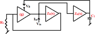
A New Generalized Approach for the Realization of Meminductor Emulator and Its Application

Nullor-Based Negative-Feedback Memristive Amplifiers: Symbolic-Oriented Modelling and Design

Universal memelement emulator using only off-the-shelf components

Data availability.

Data sharing not applicable to this article as no datasets were generated or analysed during the current study.

Code availability

Not applicable.

Y. Babacan, An operational transconductance amplifier-based memcapacitor and meminductor. Electrica 18 (1), 36–38 (2018)

MathSciNet Google Scholar

K. Bhardwaj, M. Srivastava, New electronically adjustable memelement emulator for realizing the behavior of fully-floating meminductor and memristor. Microelectron. J. 114 , 105126 (2021)

Article Google Scholar

K. Bhardwaj, M. Srivastava, New grounded passive elements-based external multiplier-less memelement emulator to realize the floating meminductor and memristor. Analog Integr. Circuits Signal Process. 110 (3), 409–429 (2022)

K. Bhardwaj, M. Srivastava, New multiplier-less compact tunable charge-controlled Memelement emulator using grounded passive elements. Circuits Syst. Signal Process. (2022). https://doi.org/10.1007/s00034-021-01895-3

K. Bhardwaj, M. Srivastava, On the boundaries of the realization of single input single element-controlled universal memelement emulator. Circuits Syst. Signal Process. 42 , 6355–6366 (2023). https://doi.org/10.1007/s00034-023-02420-4

D. Biolek, V. Bajer, V. Biolkova, Z. Kolka, Mutators for transforming nonlinear resistor into memristor, in 2011 20th European Conference on Circuit Theory and Design (ECCTD) (IEEE, 2011), pp. 488–491

D. Biolek, V. Biolkova, Mutator for transforming memristor into memcapacitor. Electron. Lett. 46 (21), 1 (2010)

D. Biolek, V. Biolková, Z. Kolka, Z. Biolek, Incremental mutators for transforming between extended higher-order elements. IEEE Trans. Circuits Syst. II Express Briefs (2024). https://doi.org/10.1109/TCSII.2024.3393471

L.O. Chua, Memristor-the missing circuit element. IEEE Trans. on Circuit Theory 18 (5), 507–519 (1971)

T. Driscoll et al., Memristive adaptive filters. Appl. Phys. Lett. 97 (9), 093502–093503 (2010)

Y. Fang, Y. Li, G. Wang, D. Gang, C. Guanrong, Complex dynamics in a memcapacitor-based circuit. Entropy 21 , 188 (2019). https://doi.org/10.3390/e21020188

Article MathSciNet Google Scholar

R. Francisco, M. Diego, A. Godoy, R. Francisco, T. Isabel, O. Akiko, R. Noel, Memcapacitor emulator based on the Miller effect. Int. J. Circuit Theory Appl. 47 , 572–579 (2019). https://doi.org/10.1002/cta.2604

S. Hasan, C. Ugur, A novel floating/grounded meminductor emulator. J. Circuits Syst. Comput. (2020). https://doi.org/10.1142/S0218126620502473

M.Z. Hosbas, F. Kaçar, A. Yesil, Memcapacitor emulator using VDTA-memristor. Analog Integr. Circuit Signal Process. 110 , 361–370 (2022). https://doi.org/10.1007/s10470-021-01974-0

M. Itoh, L. Chua, Duality of memristor circuits. Int. J. Bifurc. Chaos 23 , 1330001 (2013). https://doi.org/10.1142/S0218127413300012

F. Kaçar, A. Yeşil, S. Minaei, H. Kuntman, Positive/negative lossy/lossless grounded inductance simulators employing single VDCC and only two passive elements. AEU Int. J. Electron. C. 68 (1), 73–78 (2014)

Z.H. Lin, H.X. Wang, Image encryption based on chaos with PWL memristor in Chua’s circuit, in International Conference on Communications, Circuits and Systems (2009), pp. 964–968

Z.-H. Lin, H. Wang, Efficient image encryption using chaos-based PWL memristor. IETE Tech. Rev. 27 (4), 318–325 (2010)

S. Minaei, I.C. Goknar, M. Yildiz, E. Yuce, Memstor, memstance simulations via a versatile 4-port built with new adder and subtractor circuits. Int. J. Electron. 102 , 911–931 (2014). https://doi.org/10.1080/00207217.2014.942890

B. Muthuswamy, P. Kokate, Memristor-based chaotic circuits. IETE Tech. Rev. 26 , 417–429 (2009)

B. Muthuswamy, Implementing memristor based chaotic circuits. Int. J. Bifurc. Chaos 20 , 1335–1350 (2010)

T. Raja, S. Mourad, Digital logic implementation in memristor-based crossbars, in 2009 International Conference on Communications, Circuits and Systems (2009), pp. 939–943

R.K. Ranjan et al., Memristor Emulator Circuit using multiple output OTA and its experimental results. J. Circuits Syst. Comput. 28 , 1950166 (2019). https://doi.org/10.1142/S0218126619501664

N. Raj, P. Deepthi, Emulation of novel and electronically tunable universal mem-elements design, in 2024 21st International Conference on Electrical Engineering/Electronics, Computer, Telecommunications and Information Technology (ECTI-CON) (IEEE, 2014), pp. 1–6

F. Romero, M. Escudero, A. Medina-Garcia, D. Morales, N. Rodriguez, Meminductor emulator based on a modified Antoniou’s Gyrator circuit. Electronics 9 (9), 1407 (2020). https://doi.org/10.3390/electronics9091407

M.P. Sah, R.K. Budhathoki, C. Yang, H. Kim, Mutator-based meminductor emulator for circuit applications. Circuits Syst. Signal Process. 33 , 2363–2383 (2014)

F. Setoudeh, M.M. Dezhdar, A new design and implementation of the floating-type charge-controlled memcapacitor emulator. Majlesi J. Telecommun. Dev. 9 (2), 71–79 (2020)

Google Scholar

P.K. Sharma, R.K. Ranjan, F. Khateb, M. Kumngern, Charged controlled mem-element emulator and its application in a chaotic system. IEEE Access 8 , 171397–171407 (2020). https://doi.org/10.1109/ACCESS.2020.3024769

A. Singh, S.K. Rai, Novel meminductor emulators using operational amplifiers and their applications in chaotic oscillators. J. Circuits Syst. Comput. (2021). https://doi.org/10.1142/S0218126621502194

A. Singh, S.K. Rai, VDCC-based memcapacitor/meminductor emulator and its application in adaptive learning circuit. Iran. J. Sci. Technol. Trans. Electr. Eng. 45 , 1151–1163 (2021). https://doi.org/10.1007/s40998-021-00440-x

Z.G.C. Taşkıran, M. Sağbaş, U.E. Ayten, H. Sedef, A new universal mutator circuit for memcapacitor and meminductor elements. Int. J. Electron. Commun. 119 , 153180 (2020). https://doi.org/10.1016/j.aeue.2020.153180

K. Witrisal, A memristor-based multicarrier UWB receiver, in IEEE International Conference on UltraWideband (2009), pp 679–683

D. Yu, X. Zhao, T. Sun, H.H. Iu, T. Fernando, A simple floating mutator for emulating memristor, memcapacitor, and meminductor. IEEE Trans. Circuits Syst. II Express Briefs 67 (7), 1334–1338 (2019)

D.S. Yu, Y. Liang, H.H. Iu, Y.H. Hu, Mutator for transferring a memristor emulator into meminductive and memcapacitive circuits. Chin. Phys. B 23 (7), 070702 (2014)

F. Yuan, Y. Deng, Y. Li, A multistable generalized meminductor with coexisting stable pinched hysteresis loops. Int. J. Bifurc. Chaos 30 , 2050023 (2020). https://doi.org/10.1142/S0218127420500236

F. Yuan, Y. Deng, Y. Li, G. Wang, The amplitude, frequency and parameter space boosting in a memristor–meminductor-based circuit. Nonlinear Dyn. 96 , 389–405 (2019). https://doi.org/10.1007/s11071-019-04795-z

X. Yirong, G. Wang, H. Iu, Y. Simin, F. Yuan, A memristor–meminductor-based chaotic system with abundant dynamical behaviors. Nonlinear Dyn. 96 , 765–788 (2019). https://doi.org/10.1007/s11071-019-04820-1

Y. Yesil, Y. Babacan, F. Kacar, An electronically controllable, fully floating memristor based on active elements: DO-OTA and DVCC. Int. J. Electron. Commun. 123 , 153315 (2020)

Q. Zhao, X. Zhang, A universal emulator for memristor, memcapacitor, and meminductor and its chaotic circuit. Chaos Interdiscip. J. Nonlinear Sci. (2019). https://doi.org/10.1063/1.5081076

Download references

No applicable.

Author information

Authors and affiliations.

Department of Electronics and Communication Engineering, NIT Jamshedpur, Jamshedpur, India

Kapil Bhardwaj & Mayank Srivastava

Thin Film Electronics Lab, Faculty of Information Technology and Communication Sciences, Tampere University, Tampere, Finland

Kapil Bhardwaj

You can also search for this author in PubMed Google Scholar

Corresponding author

Correspondence to Mayank Srivastava .

Ethics declarations

Conflict of interest.

There is no conflict of interest.

Additional information

Publisher's note.

Springer Nature remains neutral with regard to jurisdictional claims in published maps and institutional affiliations.

Rights and permissions

Springer Nature or its licensor (e.g. a society or other partner) holds exclusive rights to this article under a publishing agreement with the author(s) or other rightsholder(s); author self-archiving of the accepted manuscript version of this article is solely governed by the terms of such publishing agreement and applicable law.

Reprints and permissions

About this article

Bhardwaj, K., Srivastava, M. On the Transformation of Memory-Less Non-linear Components into Memristors. Circuits Syst Signal Process (2024). https://doi.org/10.1007/s00034-024-02828-6

Download citation

Received : 05 March 2024

Revised : 04 August 2024

Accepted : 05 August 2024

Published : 20 August 2024

DOI : https://doi.org/10.1007/s00034-024-02828-6

Share this article

Anyone you share the following link with will be able to read this content:

Sorry, a shareable link is not currently available for this article.

Provided by the Springer Nature SharedIt content-sharing initiative

Non-linear capacitor
Non-linear inductor
Find a journal
Publish with us
Track your research

COMMENTS

Determining the level of evidence: Nonexperimental research ...
Humans. Research Design*. To support evidence-based nursing practice, the authors provide guidelines for appraising research based on quality, quantity, and consistency. This article, the second of a three-part series, focuses on nonexperimental research designs.
Planning and Conducting Clinical Research: The Whole Process
Experimental or non-experimental: Non-experimental research (i.e., "observational"), in contrast to experimental, involves data collection of the study participants in their natural or real-world environments. Non-experimental researches are usually the diagnostic and prognostic studies with cross-sectional in data collection.
Nonexperimental research: strengths, weaknesses and issues of precision
Nonexperimental research, defined as any kind of quantitative or qualitative research that is not an experiment, is the predominate kind of research design used in the social sciences. How to unambiguously and correctly present the results of nonexperimental research, however, remains decidedly unclear and possibly detrimental to applied ...
Quantitative Research with Nonexperimental Designs
There are two main types of nonexperimental research designs: comparative design and correlational design. In comparative research, the researcher examines the differences between two or more groups on the phenomenon that is being studied. For example, studying gender difference in learning mathematics is a comparative research.
Determining the level of evidence: Nonexperimental research ...
Metrics. Abstract. In Brief. To support evidence-based nursing practice, the authors provide guidelines for appraising research based on quality, quantity, and consistency. This article, the second of a three-part series, focuses on nonexperimental research designs. This three-part series supports and describes evidence-based practice.
Nonexperimental research: strengths, weaknesses and issues of precision
The research design is non-experimental. A non-experimental research design as defined by Reio (2016) is the predominant method researchers use in the social sciences. The design is useful when ...
PDF Non-experimental study designs: The basics and recent advances
So when we can't randomize…the role of design for non-experimental studies. •Should use the same spirit of design when analyzing non-experimental data, where we just see that some people got the treatment and others the control •Helps articulate 1) the causal question, and 2) the timing of covariates, exposure, and outcomes.
A Primer to Experimental and Nonexperimental Quantitative Research: The
There are two broad areas of inquiry in quantitative research (Fig 1).There is research that aims to describe or explore diseases, conditions, or variables; and there is research that tries to find a causal relationship among variables, conditions, and real-life situations. 2 These two fields of research do not exist independently; they talk to each other.
Using public clinical trial reports to probe non-experimental causal
Non-experimental studies (also known as observational studies) are valuable for estimating the effects of various medical interventions, but are notoriously difficult to evaluate because the methods used in non-experimental studies require untestable assumptions. This lack of intrinsic verifiability makes it difficult both to compare different non-experimental study methods and to trust the ...
Non-Experimental Comparative Effectiveness Research: How to ...
Knowledge about the benefit-to-harm balance of alternative treatment options is central to high-quality patient care. In contrast to the traditional hierarchy of evidence, led by randomized designs, the emerging consensus is to move away from judging a study's validity based only on randomization. Ethical, practical, and financial considerations dictate that most epidemiologic research be ...
Overview of Nonexperimental Research
Key Takeaways. Nonexperimental research is research that lacks the manipulation of an independent variable, control of extraneous variables through random assignment, or both. There are three broad types of nonexperimental research. Single-variable research focuses on a single variable rather than a relationship between variables.
7.1 Overview of Nonexperimental Research
Key Takeaways. Nonexperimental research is research that lacks the manipulation of an independent variable, control of extraneous variables through random assignment, or both. There are three broad types of nonexperimental research. Single-variable research focuses on a single variable rather than a relationship between variables.
Using Non-experimental Data to Estimate Treatment Effects
Second, a new area of methodological research has developed generalized propensity scores for use with non-binary treatments (5,16,39). A final concern with any non-experimental study is that of unmeasured confounding: there may be some unmeasured variable related to both which treatment an individual receives and their outcome.
Designs of Empirical Evaluations of Nonexperimental Methods in Field
Research article. First published online June 28, 2018. Designs of Empirical Evaluations of Nonexperimental Methods in Field Settings ... (2014). The performance of non-experimental designs in the evaluation of environmental programs: A design-replication study using a large-scale randomized experiment as a benchmark. Journal of Economic ...
Nonexperimental Comparative Effectiveness Research Using Linked
Comparative Effectiveness Research (CER) has gained a great deal of attention over the past year through the new federal coordinating council, 1 the recent Institute of Medicine (IOM) report, 2 and the American Recovery & Reinvestment Act (ARRA) stimulus funding. 3 CER has a broad scope as defined by the IOM, addressing "…the generation and synthesis of evidence that compares the benefits ...
Overview of Non-Experimental Research
Non-experimental research is research that lacks the manipulation of an independent variable. Rather than manipulating an independent variable, researchers conducting non-experimental research simply measure variables as they naturally occur (in the lab or real world). Most researchers in psychology consider the distinction between experimental ...
Toward a New Classification of Nonexperimental Quantitative Research
Abstract. A substantial proportion of quantitative educational research is non-experimental because many important variables of interest are not manipulable. Because nonexperimental research is an important methodology employed by many researchers, it is important to use a classification system of nonexperimental methods that is highly ...
6.1 Overview of Non-Experimental Research
Non-experimental research is research that lacks the manipulation of an independent variable. Rather than manipulating an independent variable, researchers conducting non-experimental research simply measure variables as they naturally occur (in the lab or real world). Most researchers in psychology consider the distinction between experimental ...
6: Non-Experimental Research
6.3: Correlational Research. Correlational research is a type of non-experimental research in which the researcher measures two variables and assesses the statistical relationship (i.e., the correlation) between them with little or no effort to control extraneous variables. There are many reasons that researchers interested in statistical ...
Research study designs: Non-experimental
The category of non-experimental designs is the most heterogeneous of the three classification categories (experimental, quasi-experimental, and non-experimental). Examples of the most common non-experimental designs are listed in Table 1. Although, in general, this category has the lowest level of scientific rigor, each design within this category varies as to its own individual level of ...
6.1: Overview of Non-Experimental Research
Non-experimental research is research that lacks the manipulation of an independent variable. Rather than manipulating an independent variable, researchers conducting non-experimental research simply measure variables as they naturally occur (in the lab or real world). Most researchers in psychology consider the distinction between experimental ...
Non-experimental research: What it is, Types & Tips
Non-experimental research is the type of research that lacks an independent variable. Instead, the researcher observes the context in which the phenomenon occurs and analyzes it to obtain information. Unlike experimental research, where the variables are held constant, non-experimental research happens during the study when the researcher ...
Experimental and Non-Experimental Methods
The goal of KQ 4 was to describe experimental and non-experimental methods in terms of study design and analytic approach. Key Findings Of the 294 studies included in this review, 156 were natural experiment studies (53%), 118 were experimental studies (40%), and 20 provided insufficient information to determine if a natural experiment took ...
Experimental research on the horizontally getting together ...
This study aims at the controllability of acoustically manipulated non-contact aggregation of bi-particle. Based on the acoustic wave radiation model of the transducer and the acoustic wave ...
Identification of circulating tumor cells captured by the FDA-cleared
Circulating Tumor Cells (CTCs) may serve as a non-invasive source of tumor material to investigate an individual's disease in real-time. The Parsortix® PC1 System, the first FDA-cleared medical device for the capture and harvest of CTCs from peripheral blood of metastatic breast cancer (MBC) patients for use in subsequent user-validated downstream analyses, enables the epitope-independent ...
On the Transformation of Memory-Less Non-linear Components into
The passive non-linear components, such as capacitors and inductors, lack inherent memory, thus limiting their applications to circuit functions like chaotic oscillators and waveform generators. In this research, it has been explored that these non-linear capacitors/inductors (NLC/I) may be transformed into functional memelements through appropriate modifications to the circuit configuration ...

Save citation to file

Add to My Bibliography

Determining the level of evidence: Nonexperimental research designs

Similar articles

Related information

Other Literature Sources

To read this content please select one of the options below:

Design/methodology/approach

Originality/value

Related articles

Report an issue or find answers to frequently asked questions

Secondary Logo

Determining the level of evidence

Full Text Access for Subscribers:

Institutional Users

Readers Of this Article Also Read

Using public clinical trial reports to probe non-experimental causal inference methods

Conclusions

Related work

The primary data source: ClinicalTrials.gov

Extracting trials with an active comparator design

Empirical Bayes effect size estimation

Effect size ranking and subsetting

Evaluation: concordant sign rate

Case study on Optum’s Clinformatics

Comparison to prior work

Importance of clinical trial filtering

Availability of data and materials

Acknowledgements

Author information

Contributions

Corresponding author

Ethics declarations

Consent for publication

Competing interests

Additional information

Rights and permissions

About this article

Share this article

BMC Medical Research Methodology

Overview of Nonexperimental Research

What Is Nonexperimental Research?

When to Use Nonexperimental Research

Types of Nonexperimental Research

Internal Validity Revisited

Share This Book

7.1 Overview of Nonexperimental Research

What Is Nonexperimental Research?

When to Use Nonexperimental Research

Types of Nonexperimental Research

Internal Validity Revisited

Key Takeaways

28 Overview of Non-Experimental Research

What Is Non-Experimental Research?

When to Use Non-Experimental Research

Types of Non-Experimental Research

Cross-Sectional, Longitudinal, and Cross-Sequential Studies

Internal Validity Revisited

Share This Book

6.1 Overview of Non-Experimental Research

What Is Non-Experimental Research?

When to Use Non-Experimental Research

Types of Non-Experimental Research

Internal Validity Revisited

Key Takeaways

Share This Book

Non-experimental research: What it is, overview & advantages

Characteristics of non-experimental research

Types of non-experimental research

When to use non-experimental research

Advantages and disadvantages

Difference between experimental and non-experimental research

MORE LIKE THIS

Customer Experience Lessons from 13,000 Feet — Tuesday CX Thoughts

Insight: Definition & meaning, types and examples

Employee Loyalty: Strategies for Long-Term Business Success

Jotform vs SurveyMonkey: Which Is Best in 2024

Other categories

Methods for Evaluating Natural Experiments in Obesity: Systematic Evidence Review [Internet].

Key Findings