problem solving circle graphs

One to one maths interventions built for KS4 success

Weekly online one to one GCSE maths revision lessons now available

In order to access this I need to be confident with:

This topic is relevant for:

Circle Graph

Here we will learn about circle graphs , including how to recognise them and how to sketch them. We will also look at solving coordinate geometry questions involving circle graphs.

There are also circle graphs worksheets based on Edexcel, AQA and OCR exam questions, along with further guidance on where to go next if you’re still stuck.

What is a circle graph?

A circle graph is the graph of an equation which forms a circle.

To do this we have a circle with radius r and centre (0, 0) .  Using Pythagoras’ Theorem it gives the general equation:

E.g. This circle has a radius of 3 so has the equation:

Which simplifies to:

How to recognise the equation of a circle

In order to recognise the equation of a circle:

Identify an x^2 term and a y^2 term

Check the radius and use r^2

Identify your final answer

Circle graph worksheet

Get your free circle graph worksheet of 20+ questions and answers. Includes reasoning and applied questions.

Related lessons on types of graphs

Circle graph is part of our series of lessons to support revision on types of graphs . You may find it helpful to start with the main types of graphs lesson for a summary of what to expect, or use the step by step guides below for further detail on individual topics. Other lessons in this series include:

• Types of graphs
• Reciprocal graph
• Exponential graph
• Cubic graph
• Straight line graph
• Quadratic graph

Circle graph examples

Example 1: recognise the equation of a circle.

Identify the correct equation for the graph:

The equation y=x^2+6 only has an x^2 term and is a quadratic function.

The equation y=x^2+12 only has an x^2 term and is also a quadratic function.

Both the equation x^2+y^2=36 and the equation x^2+y^2=12 have an x^2 term and a y^2 term.

2 Check the radius and use r^2

The radius of the circle is 6 , so

3 Identify your final answer

The correct equation for the graph is:

Example 2: recognise the equation of a circle

The equation y=x^2+20 only has an x^2 term and is a quadratic function.

The equation y=x^3+10 only has an x^3 term and is a cubic function.

Both the equation x^2+y^2=20 and the equation x^2+y^2=100 have an x^2 term and a y^2 term.

The radius of the circle is 10 , so

How to sketch a circle graph

In order to sketch a circle graph:

Check the radius

Draw a circle with centre (0, 0)

Label where the circle crosses the axes

Explain how to sketch a circle graph

Sketching a circle graph examples

Example 3: sketching a circle graph.

Sketch x^2+y^2=64

The equation of a circle graph with centre (0, 0) is of the form:

Example 4: sketching a circle graph

Sketch x^2+y^2=144

How to find the equation of a tangent to a circle

In order to find the equation of a tangent to a circle:

Find the gradient of the radius from the given point to the centre

Find the gradient of the perpendicular

Find the equation of the lines using the gradient and the given point

Write the equation of the tangent

Finding the equation of a tangent to a circle examples

Example 5: finding the equation of a tangent to a circle.

Find the equation of the tangent to the circle x^2+y^2=90 at the point (9,3)

The gradient of the radius is:

The radius and the tangent meet at right angles; this is a circle theorem . Therefore the radius and the tangent are perpendicular .

The product of perpendicular gradients is −1 .

So the gradient of the tangent is:

The equation of a straight line is of the form:

We can substitute the original point for the x and y values. The gradient of the tangent is the value of m .  We can then work out c .

Example 6: finding the equation of a tangent to a circle

Find the equation of the tangent to the circle x^2+y^2=13 at the point (-3,2)

Common misconceptions

• Make sure that you use r^2

The equation of the circle requires the radius NOT the diameter. Remember the radius is half the diameter.

• The radius is always a positive number

Since the radius is a length it is always positive. E.g. The radius of this circle is 12 and r^2=144 . The equation of this circle is x^2+y^2=144

Practice circle graph questions

1. What is the equation for this graph:

The equation of a circle graph with centre (0,0) is of the form:

The radius of the circle is 5 , so

2. What is the equation for this graph:

The radius of the circle is 7 , so

The equation of a circle graph with the centre of the circle (0,0) is of the form:

So we draw a circle with centre (0,0) radius of the circle is 4.

5. Find the equation of the tangent to the circle x^2+y^2=80 at the point (8,4)

The gradient of the tangent will be: -2

So the equation would be:

6. Find the equation of the tangent to the circle x^2+y^2=20 at the point (-2, 4)

The gradient of the tangent will be: \frac{1}{2}

Circle graph GCSE questions

1.   Identify the equation of this graph:

The correct equation is:

2.   A point P (2,4) lies on the circle with equation:

Find the equation of the tangent to the circle at the point P.

Gradient of OP, the radius is 2

The gradient of the tangent is -\frac{1}{2}

The equation of the tangent is:

3.   (a)  On the grid, draw the graph of:

(b) Hence find estimates for the solutions of simultaneous equations:

for a circle with centre (0.0)

for the correct circle with radius 4

x=3.9 and y= -0.9

x= -3.9 and y=0.9

for drawing the line graph x+y=3

for one of the correct pair of x and y solutions OR both x -values OR both y -values

for both pairs of correct solutions

Learning checklist

You have now learned how to:

• recognise the equation of a circle with centre at the origin
• use the equation of a circle with centre at the origin
• find the equation of a tangent to a circle at a given point

The next lessons are

• Factorising
• Solving equations

Still stuck?

Prepare your KS4 students for maths GCSEs success with Third Space Learning. Weekly online one to one GCSE maths revision lessons delivered by expert maths tutors.

Find out more about our GCSE maths tuition programme.

Privacy Overview

Circle Equations

A circle is easy to make:

Draw a curve that is "radius" away from a central point.

All points are the same distance from the center.

In fact the definition of a circle is

Circle: The set of all points on a plane that are a fixed distance from a center.

Circle on a Graph

Let us put a circle of radius 5 on a graph:

Now let's work out exactly where all the points are.

We make a right-angled triangle:

And then use Pythagoras :

x 2 + y 2 = 5 2

There are an infinite number of those points, here are some examples:

In all cases a point on the circle follows the rule x 2 + y 2 = radius 2

We can use that idea to find a missing value

Example: x value of 2, and a radius of 5

(The ± means there are two possible values: one with + the other with − )

And here are the two points:

More General Case

Now let us put the center at (a,b)

So the circle is all the points (x,y) that are "r" away from the center (a,b) .

Now lets work out where the points are (using a right-angled triangle and Pythagoras ):

It is the same idea as before, but we need to subtract a and b :

(x−a) 2 + (y−b) 2 = r 2

And that is the "Standard Form" for the equation of a circle!

It shows all the important information at a glance: the center (a,b) and the radius r .

Example: A circle with center at (3,4) and a radius of 6:

Start with:

Put in (a,b) and r:

(x−3) 2 + (y−4) 2 = 6 2

We can then use our algebra skills to simplify and rearrange that equation, depending on what we need it for.

Try it Yourself

"general form".

But you may see a circle equation and not know it !

Because it may not be in the neat "Standard Form" above.

As an example, let us put some values to a, b and r and then expand it

And we end up with this:

x 2 + y 2 − 2x − 4y − 4 = 0

It is a circle equation, but "in disguise"!

So when you see something like that think "hmm ... that might be a circle!"

In fact we can write it in "General Form" by putting constants instead of the numbers:

x 2 + y 2 + Ax + By + C = 0

Note: General Form always has x 2 + y 2 for the first two terms .

Going From General Form to Standard Form

Now imagine we have an equation in General Form :

How can we get it into Standard Form like this?

The answer is to Complete the Square (read about that) twice ... once for x and once for y :

Example: x 2 + y 2 − 2x − 4y − 4 = 0

Now complete the square for x (take half of the −2, square it, and add to both sides):

(x 2 − 2x + (−1) 2 ) + (y 2 − 4y) = 4 + (−1) 2

And complete the square for y (take half of the −4, square it, and add to both sides):

(x 2 − 2x + (−1) 2 ) + (y 2 − 4y + (−2) 2 ) = 4 + (−1) 2 + (−2) 2

And we have it in Standard Form!

(Note: this used the a=1, b=2, r=3 example from before, so we got it right!)

Unit Circle

If we place the circle center at (0,0) and set the radius to 1 we get:

How to Plot a Circle by Hand

1. Plot the center (a,b)

2. Plot 4 points "radius" away from the center in the up, down, left and right direction

3. Sketch it in!

Example: Plot (x−4) 2 + (y−2) 2 = 25

The formula for a circle is (x−a) 2 + (y−b) 2 = r 2

So the center is at (4,2)

And r 2 is 25 , so the radius is √25 = 5

So we can plot:

• The Center: (4,2)
• Up: (4,2+5) = (4,7)
• Down: (4,2−5) = (4,−3)
• Left: (4−5,2) = (−1,2)
• Right: (4+5,2) = (9,2)

Now, just sketch in the circle the best we can!

How to Plot a Circle on the Computer

We need to rearrange the formula so we get "y=".

We should end up with two equations (top and bottom of circle) that can then be plotted.

So the center is at (4,2) , and the radius is √25 = 5

Rearrange to get "y=":

So when we plot these two equations we should have a circle:

• y = 2 + √[25 − (x−4) 2 ]
• y = 2 − √[25 − (x−4) 2 ]

Try plotting those functions on the Function Grapher .

It is also possible to use the Equation Grapher to do it all in one go.

How To Graph a Circle

Graphing a circle

Graphing circles  requires two things: the coordinates of the center point, and the radius of a circle. A circle is the set of all points the same distance from a given point, the center of the circle. A radius,  r , is the distance from that center point to the circle itself.

On a graph, all those points on the circle can be determined and plotted using (x,y)  coordinates.

Circle equations

Two expressions show how to plot a circle: the  center-radius form  and the  standard form . Where  x  and  y  are the coordinates for all the circle's points,  h  and  k  represent the center point's  x  and  y  values, with  r  as the radius of the circle

Center-radius form

The center-radius form looks like this:

Standard equation of a circle

The standard, or general, form requires a bit more work than the center-radius form to derive and graph. The standard form equation looks like this:

In the general form,  D ,  E , and  F  are given values, like integers, that are coefficients of the  x  and  y  values.

Using the center-radius form {use-crf}

If you are unsure that a suspected formula is the equation needed to graph a circle, you can test it. It must have four attributes:

The x and y terms must be squared.

All terms in the expression must be positive (which squaring the values in parentheses will accomplish).

The center point is given as (h,k) , the x and y coordinates.

The value for r , radius, must be given and must be a positive number (which makes common sense; you cannot have a negative radius measure).

The center-radius form gives away a lot of information to the trained eye. By grouping the  h  value with the  x ( x − h ) 2 x{\left(x-h\right)}^{2} x ( x − h ) 2 , the form tells you the  x  coordinate of the circle's center. The same holds for the kk value; it must be the  y  coordinate for the center of your circle.

Once you ferret out the circle's center point coordinates, you can then determine the circle's radius,  r . In the equation, you may not see  r 2 {r}^{2} r 2 , but a number, the square root of which is the actual radius.

With luck, the squared  r  value will be a whole number, but you can still find the square root of decimals using a calculator.

Which are center-radius form?

Try these seven equations to see if you can recognize the center-radius form. Which ones are center-radius, and which are just line or curve equations?

( x − 2 ) 2 + ( y − 3 ) 2 = 16 {\left(x-2\right)}^{2}+{\left(y-3\right)}^{2}=16 ( x − 2 ) 2 + ( y − 3 ) 2 = 16

5 x + 3 y = 6 5x+3y=6 5 x + 3 y = 6

( x + 1 ) 2 + ( y + 1 ) 2 = 25 {\left(x+1\right)}^{2}+{\left(y+1\right)}^{2}=25 ( x + 1 ) 2 + ( y + 1 ) 2 = 25

y = 6 x + 2 y=6x+2 y = 6 x + 2

( x + 4 ) 2 + ( y − 6 ) 2 = 49 {\left(x+4\right)}^{2}+{\left(y-6\right)}^{2}=49 ( x + 4 ) 2 + ( y − 6 ) 2 = 49

( x − 5 ) 2 + ( y + 9 ) 2 = 8.1 {\left(x-5\right)}^{2}+{\left(y+9\right)}^{2}=8.1 ( x − 5 ) 2 + ( y + 9 ) 2 = 8.1

y = x 2 + − 6 x + 3 y={x}^{2}+-6x+3 y = x 2 + − 6 x + 3

Only equations 1, 3, 5 and 6 are center-radius forms.  The second equation graphs a straight line; the fourth equation is the familiar slope-intercept form; the last equation graphs a parabola.

How to graph a circle equation

A circle can be thought of as a graphed line that curves in both its  x  and  y  values. This may sound obvious, but consider this equation:

Here the  x  value alone is squared, which means we will get a curve, but only a curve going up and down, not closing back on itself. We get a parabolic curve, so it heads off past the top of our grid, its two ends never to meet or be seen again.

Introduce a second x-value exponent, and we get more lively curves, but they are, again, not turning back on themselves.

The curves may snake up and down the y-axis as the line moves across the x-axis, but the graphed line is still not returning on itself like a snake biting its tail.

To get a curve to graph as a circle, you need to change  both  the  x exponent  and  the  y exponent. As soon as you take the square of both  x  and  y  values, you get a circle coming back unto itself!

Often the center-radius form does not include any reference to measurement units like mm, m, inches, feet, or yards. In that case, just use single grid boxes when counting your radius units.

Center at the origin

When the center point is the origin  (0, 0)  of the graph, the center-radius form is  greatly  simplified:

For example, a circle with a radius of 7 units and a center at  (0, 0)  looks like this as a formula and a graph:

How to graph a circle using standard form

If your circle equation is in  standard or general form , you must first  complete the square  and then work it into center-radius form. Suppose you have this equation:

Rewrite the equation so that all your x-terms are in the first parentheses and y-terms are in the second:

You have isolated the constant to the right and added the values  ? 1 {?}_{1} ? 1 ​  and  ? 2 {?}_{2} ? 2 ​  to both sides. The values  ? 1 {?}_{1} ? 1 ​  and  ? 2 {?}_{2} ? 2 ​  are each the number you need in each group to complete the square.

Take the coefficient of  x and divide by 2 . Square it. That is your new value for ? 1 {?}_{1} ? 1 ​ :

Repeat this for the value to be found with the y-terms:

Replace the unknown values  ? 1 {?}_{1} ? 1 ​ and  ? 2 {?}_{2} ? 2 ​  in the equation with the newly calculated values:

You now have the center-radius form for the graph. You can plug the values in to find this circle with center point  (-4, 3)  and a radius of  5.385 units (the square root of 29 ):

Cautions to look out for

In practical terms, remember that the center point, while needed, is not actually part of the circle. So, when actually graphing your circle, mark your center point very lightly. Place the easily counted values along the  x and  y  axes, by simply counting the radius length along the horizontal and vertical lines.

If precision is not vital, you can sketch in the rest of the circle. If precision matters, use a ruler to make additional marks, or a drawing compass to swing the complete circle.

You also want to mind your negatives. Keep careful track of your negative values, remembering that, ultimately, the expressions must all be positive (because your x-values and y-values are squared).

A free service from Mattecentrum

Circle graphs

• Circle graphs I
• Circle graphs II
• Circle graphs III

A circle is the same as 360°. You can divide a circle into smaller portions. A part of a circle is called an arc and an arc is named according to its angle.

A circle graph, or a pie chart, is used to visualize information and data. A circle graph is usually used to easily show the results of an investigation in a proportional manner. The arcs of a circle graph are proportional to how many percent of population gave a certain answer.

An investigation was made in Mathplanet high school to investigate what color of jeans was the most common among the students. This circle graph shows how many percent of the school had a certain color. We now want to know how many angles each percentage corresponds to.

To find out the number of degrees for each arc or section in the graph we multiply the percentage by 360°.

$$Blue\: 57\%: 0.57\cdot 360^{\circ}=205.2^{\circ}$$

$$Black\: 19\%:0.19\cdot 360^{\circ}=68.4^{\circ}$$

$$Beige\: 12\%:0.12\cdot 360^{\circ}=43.2^{\circ}$$

$$Grey\: 8\%:0.08\cdot 360^{\circ}=28.8^{\circ}$$

$$Red\: 4\%:0.04\cdot 360^{\circ}=14.4^{\circ}$$

When we want to draw a circle graph by ourselves we need to rewrite the percentages for each category into degrees of a circle and then use a protractor to make the graph.

If we ask 100 persons which TV program they like the most, we get this result.

We know that the total amount of persons is 100. Now we need to find the ratio for each TV program.

$$GA:\frac{17}{100}=0.17$$

$$FG: \frac{34}{100}=0.34$$

$$TB:\frac{15}{100}=0.15$$

$$GG:\frac{26}{100}=0.26$$

$$AFV:\frac{8}{100}=0.08$$

To find the degrees of each TV program we multiply by 360.

$$GA:0.17\cdot 360^{\circ}=61.2^{\circ}$$

$$FG: 0.34\cdot 360^{\circ}=122.4^{\circ}$$

$$TB:0.15\cdot360^{\circ}= 54^{\circ}$$

$$GG:0.26\cdot 360^{\circ}=93.6^{\circ}$$

$$AFV:0.08\cdot 360^{\circ}=28.8^{\circ}$$

And then we use a protractor to draw the chart. It will look something like this:

Video lesson

Find the values in degrees

• Pre-Algebra
• Measure areas
• Pyramids, prisms, cylinders and cones
• Square roots and real numbers
• The Pythagorean Theorem
• Trigonometry
• Algebra 1 Overview
• Algebra 2 Overview
• Geometry Overview
• SAT Overview
• ACT Overview

Equation of a Circle Practice Questions

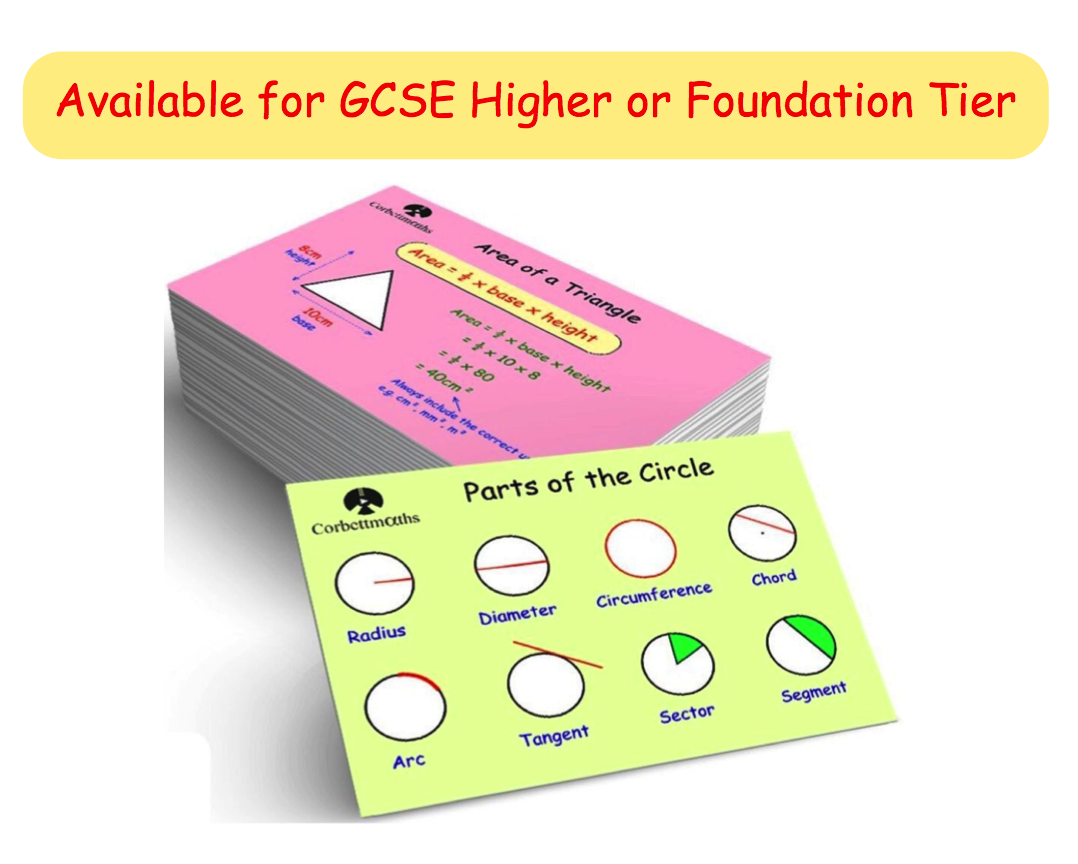
Click here for questions, click here for answers, gcse revision cards.

5-a-day Workbooks

Primary Study Cards

Privacy Policy

Terms and Conditions

Corbettmaths © 2012 – 2024

If you're seeing this message, it means we're having trouble loading external resources on our website.

If you're behind a web filter, please make sure that the domains *.kastatic.org and *.kasandbox.org are unblocked.

To log in and use all the features of Khan Academy, please enable JavaScript in your browser.

Statistics and probability

Course: statistics and probability   >   unit 1.

• Identifying individuals, variables and categorical variables in a data set
• Individuals, variables, and categorical & quantitative data
• Reading pictographs
• Read picture graphs (multi-step problems)
• Reading bar graphs
• Reading bar graphs: Harry Potter
• Creating a bar graph
• Create bar graphs
• Reading bar charts: comparing two sets of data
• Read bar graphs (2-step problems)
• Reading bar charts: putting it together with central tendency

Reading pie graphs (circle graphs)

• Picture graphs (pictographs) review
• Bar graphs review

Want to join the conversation?

• Upvote Button navigates to signup page
• Downvote Button navigates to signup page
• Flag Button navigates to signup page

Video transcript

Circle Graphs

Math can be as easy as pie—charts! Here are printable teaching ideas, circle-graph worksheets, activities, and independent practice pages to build skills at multiple levels for reading and interpreting circle graphs and representing data visually. Great for problem solving and for teaching fractions and probability.

TRY US RISK-FREE FOR 30 DAYS!

ADD TO YOUR FILE CABINET

THIS RESOURCE IS IN PDF FORMAT

Printable Details

• Number of pages:
• Guided Reading Level:
• Common Core:

Number Line

• circle\:(0,\:0),\:r=5
• circle\:(1,\:4),\:d=10
• c(-1,\:-4),\:d=6
• (0,\:5),\:r=8

circle-equation-calculator

• Practice, practice, practice Math can be an intimidating subject. Each new topic we learn has symbols and problems we have never seen. The unknowing...

Please add a message.

Message received. Thanks for the feedback.

• Search Menu
• Sign in through your institution
• Advance articles
• Author Guidelines
• Submission Site
• Open Access
• Why publish with this journal?
• About Bioinformatics
• Journals Career Network
• Editorial Board
• Advertising and Corporate Services
• Self-Archiving Policy
• Dispatch Dates
• Journals on Oxford Academic
• Books on Oxford Academic

Article Contents

Kragen: a knowledge graph-enhanced rag framework for biomedical problem solving using large language models.

• Article contents
• Figures & tables
• Supplementary Data

Nicholas Matsumoto, Jay Moran, Hyunjun Choi, Miguel E Hernandez, Mythreye Venkatesan, Paul Wang, Jason H Moore, KRAGEN: a knowledge Graph-Enhanced RAG framework for biomedical problem solving using large language models, Bioinformatics , 2024;, btae353, https://doi.org/10.1093/bioinformatics/btae353

• Permissions Icon Permissions

Answering and solving complex problems using a large language model (LLM) given a certain domain such as biomedicine is a challenging task that requires both factual consistency and logic, and LLMs often suffer from some major limitations, such as hallucinating false or irrelevant information, or being influenced by noisy data. These issues can compromise the trustworthiness, accuracy, and compliance of LLM-generated text and insights.

KRAGEN (Knowledge Retrieval Augmented Generation ENgine) is a new tool that combines knowledge graphs, Retrieval Augmented Generation (RAG), and advanced prompting techniques to solve complex problems with natural language. KRAGEN converts knowledge graphs into a vector database and uses RAG to retrieve relevant facts from it. KRAGEN uses advanced prompting techniques: namely graph-of-thoughts (GoT), to dynamically break down a complex problem into smaller subproblems, and proceeds to solve each subproblem by using the relevant knowledge through the RAG framework, which limits the hallucinations, and finally, consolidates the subproblems and provides a solution. KRAGEN’s graph visualization allows the user to interact with and evaluate the quality of the solution’s GoT structure and logic.

KRAGEN is deployed by running its custom Docker containers. KRAGEN is available as open-source from GitHub at: https://github.com/EpistasisLab/KRAGEN .

[email protected]

Email alerts

Citing articles via, looking for your next opportunity.

• Recommend to your Library

Affiliations

• Online ISSN 1367-4811
• Copyright © 2024 Oxford University Press
• About Oxford Academic
• Publish journals with us
• University press partners
• What we publish
• New features  
• Open access
• Institutional account management
• Rights and permissions
• Get help with access
• Accessibility
• Advertising
• Media enquiries
• Oxford University Press
• Oxford Languages
• University of Oxford

Oxford University Press is a department of the University of Oxford. It furthers the University's objective of excellence in research, scholarship, and education by publishing worldwide

• Copyright © 2024 Oxford University Press
• Cookie settings
• Cookie policy
• Privacy policy
• Legal notice

This Feature Is Available To Subscribers Only

Sign In or Create an Account

This PDF is available to Subscribers Only

For full access to this pdf, sign in to an existing account, or purchase an annual subscription.

Learning Topological Representations with Bidirectional Graph Attention Network for Solving Job Shop Scheduling Problem - Author Response

1 general resposne, 1.1 regarding the comparison against cp-sat..

Both reviewers #77C8 and #tkEw commented that the performance of our method is inferior to that of CP-SAT. Therefore, we should address this concern in the general response to benefit all the reviewers and audiences.

Specifically, we show that the proposed method outperforms CP-SAT by a large margin on the extremely large instances containing at least 8000 operations.

CP-SAT is a constraint programming solver that uses SAT methods and is known for taking a lot of time to find optimal solutions [AR1]. In comparison, our approach is an improvement heuristic that prioritizes quickly finding high-quality solutions. This makes CP-SAT more suitable for smaller instances that do not require extensive computational time.

[AR1] https://developers.google.com/optimization/cp

1.2 Regarding the updated version of the manuscript

Please be informed that we are working on the updated version of the manuscript to accommodate all the comments and correct possible errors, which will be uploaded soon.

Meanwhile, we respond to all the reviewers’ comments to facilitate discussion. We have tried to make the responses informative enough for discussion without referring to the revised manuscript.

We remain committed to further refining it as necessary up until the point of publication.

2 Response to Reviewer EAgF

We thank the reviewer for the time and effort in reviewing our paper.

2.1 Reproducibility is poor.

Responses : As mentioned in the ‘Experiment Setup’ section, Appendix E includes the detailed configurations, including hyperparameters for the proposed neural network, training, and testing configurations. We also guarantee that our code will be published once the paper is accepted.

2.2 The last paragraph of the "related literature" is missing some recent works in the space of gnns for graph attention.

Responses : We thank the reviewer for indicating the limitations of the literature review. We want to clarify that this paper’s main contribution is to propose a novel end-to-end learning-based improvement heuristic method to solve the JSSP problem. The target is not to design a GNN structure that outperforms all recent GNN baselines. As an example in the following paper:

[AR2] Ni, Fei, et al. "A multi-graph attributed reinforcement learning based optimization algorithm for large-scale hybrid flow shop scheduling problem." Proceedings of the 27th ACM SIGKDD Conference on Knowledge Discovery & Data Mining. 2021.

The literature review in [AR2] mainly focuses on approaches for scheduling problems rather than the GNN itself.

Furthermore, the first paper referred by the reviewer:

[WWW 2019] Heterogeneous Graph Attention Network. In The World Wide Web Conference (WWW ’19). Association for Computing Machinery, New York, NY, USA, 2022–2032. https://doi.org/10.1145/3308558.3313562

The proposed HAN network in this paper heavily relies on the random-walk-based sampling approaches for neighbourhood message aggregation, which is unsuitable for JSSP for the following reasons. For any disjunctive graph, each operation will have the predecessor and successor nodes modelling the precedent constraints and processing orders among machines. Sampling the neighbours via random walks will easily neglect any of the two aspects of information. Missing this critical information will lead to inferior performance.

For the second literature pointed out by the reviewer:

[IEEE ICDM 2021] "Bi-Level Attention Graph Neural Networks," 2021 IEEE International Conference on Data Mining (ICDM), Auckland, New Zealand, 2021, pp. 1126-1131, doi: 10.1109/ICDM51629.2021.00133.

It is not guaranteed that the Bi-level attention GNN poses linear computational complexity as TBGAT proposed in our paper, which is an important factor in evaluating a (neural-)solver for combinatorial optimization problems like JSSP.

Nonetheless, we have added the two pieces of literature mentioned by the reviewer in the literature review.

2.3 The authors need to provide more motivation as to why the jssp problem is important to investigate since the current writing does not reflect this.

Responses : We thank the reviewer for this comment. The updated version of the Introduction section explains why JSSP is worth investigating.

2.4 Can the authors also more clearly indicate what the contributions (of novelty) for their work are?

We summarize the contributions as follows:

1. We propose a novel bidirectional graph attention network (TBGAT) tailored for disjunctive graphs, effectively capturing their unique topological features, which utilizes two independent graph attention modules to learn forward and backward views and incorporate forward and backward topological sorts.

2. We demonstrate that forward topological order in disjunctive graphs corresponds to global processing orderings and present an algorithm for efficient GPU computation.

3. We design an entropy-regularized REINFORCE algorithm to facilitate exploration during training effectively.

4. Theoretical analysis and experiments demonstrate that TBGAT’s linear computational complexity regarding the number of jobs and machines is a key attribute for practical JSSP solving.

5. According to comprehensive experimental results, we achieved new state-of-the-art (SOTA) performance across all datasets, significantly surpassing all neural baselines.

3 Response to Reviewer 6hRG

We really appreciate Reviewer 6hRG’s careful examination and detailed comments, which help us improve the manuscript’s clarity. Here, we present our response to each comment.

3.1 Regarding the error in figure 1.

We thank the reviewer for pointing out this error. However, the definition here for ‘longest’ is not based on the number of nodes but on the total processing time of all operations along the path. Please refer to the quote “The critical path (or paths) is the longest path (in time) from Start to Finish; it indicates the minimum time necessary to complete the entire project.” in the following article for clarification:

[AR3] https://hbr.org/1963/09/the-abcs-of-the-critical-path-method

Therefore, according to the critical path definition, the path shown in Figure 1 (c) can indeed be a critical path, given that the total processing time of all the operations on the path is the largest among all paths from S to T.

We have updated the definition of the critical path to clarify the misleading.

Again, Thank you for the thorough review and finding of this subtle error.

3.2 Regarding the latest starting time L ⁢ S ⁢ T i ⁢ j 𝐿 𝑆 subscript 𝑇 𝑖 𝑗 LST_{ij} italic_L italic_S italic_T start_POSTSUBSCRIPT italic_i italic_j end_POSTSUBSCRIPT and L ⁢ S ⁢ T m ⁢ k 𝐿 𝑆 subscript 𝑇 𝑚 𝑘 LST_{mk} italic_L italic_S italic_T start_POSTSUBSCRIPT italic_m italic_k end_POSTSUBSCRIPT for operations O i ⁢ j subscript 𝑂 𝑖 𝑗 O_{ij} italic_O start_POSTSUBSCRIPT italic_i italic_j end_POSTSUBSCRIPT and O m ⁢ k subscript 𝑂 𝑚 𝑘 O_{mk} italic_O start_POSTSUBSCRIPT italic_m italic_k end_POSTSUBSCRIPT in Corollary 1.

Responses : Yes, you are correct. According to the definition of L ⁢ S ⁢ T 𝐿 𝑆 𝑇 LST italic_L italic_S italic_T in equation (2), it should be L ⁢ S ⁢ T j ⁢ i < L ⁢ S ⁢ T m ⁢ k 𝐿 𝑆 subscript 𝑇 𝑗 𝑖 𝐿 𝑆 subscript 𝑇 𝑚 𝑘 LST_{ji}<LST_{mk} italic_L italic_S italic_T start_POSTSUBSCRIPT italic_j italic_i end_POSTSUBSCRIPT < italic_L italic_S italic_T start_POSTSUBSCRIPT italic_m italic_k end_POSTSUBSCRIPT

3.3 In the paragraph just below Corollary 1, the authors use "DRL" without defining it first.

Responses : We thank the reviewer for identifying this ill-defined abbreviation. We have added the term ‘DRL’ to the Introduction.

3.4 Regarding the error in the paragraph defining the message-passing operator.

Responses : We thank the reviewer for identifying this mistake. We have corrected the mistake in the main paper.

3.5 Regarding the naming error in figure 5.

Responses : We thank the reviewer for identifying this mistake. We have corrected the mistake in Figure 5.

3.6 Regarding the reference index error of Appendix F in Section 5.4.

Responses : We thank the reviewer for identifying this subtle indexing error. We have corrected the mistake accordingly.

4 Response to Reviewer 77C8

We appreciate the reviewer’s acknowledgement of our research. We will address each of the concerns raised by the reviewer in our response.

4.1 Not really a weakness of the work, but the problem is that it remains NP-hard. In some np-hard problems the inputs appearing in practice practically always are solvable in polynomial time. But not here, I guess. The proposed solution has amazing speed, but if I read the tables correctly, I can see that CP-SAT tends to produce better solutions.

Responses : We kindly refer the reviewer to the general response, where we have provided an experiment to show that our method is superior to CP-SAT for extremely large instances.

5 Response to Reviewer tkEw (7)

We are grateful for the reviewer’s recognition of our study.

5.1 How are the two GNNs trained? In particular, what is the loss function used by both FEM and BEM? This must be clearly described.

Responses : The detailed training procedure, including the input, output, and loss function, is clearly described in Algorithm 1 in Appendix D. Due to the page limit for the submission version, we have included Algorithm 1 as an appendix. As the final version of the paper will be two pages longer, we will move the training strategy to the main paper.

5.2 Framework is trained for a given instance size (different instance sizes require different trained models).

Responses : We thank the reviewer for allowing us to answer this question. Even though we do not explicitly elaborate in the manuscript, our policy network can process a batch of disjunctive graphs with different problem sizes, i.e., the number of nodes, due to the GNN network that can naturally process a batch of graphs of various sizes, the proposed TBGAT network inherits such characteristics. The proposed MPTS operator also guarantees the calculation of topological features of graphs with different sizes within a batch, further facilitating batch processing. In summary, our proposed methods can be learned and tested on a batch of JSSP instances of diverse sizes.

5.3 It is a bit disappointing that the proposed framework cannot produce optimal results obtained by mathematical programming CP-SAT even on small instances when CP-SAT requires very little time. It would be interesting to understand why is this the case. Is there some other important inherent structure that CP-SAT is exploring that is not being captured by this neural-based framework?

Responses : We kindly redirect you to the general response above for detailed explanations. The CP-SAT method is a constraint programming solver that uses SAT (satisfiability) methods for finding the optimal solutions, consuming a massive amount of time [AR4]. Our method is an improvement heuristic searching for high-quality solutions in a limited time. Therefore, CP-SAT is more suitable for instances that are not extremely large. In the general response, we will show that our method outperforms CP-SAT by a large margin for extremely large instances (always witnessed in real manufacturing industries).

[AR4] https://developers.google.com/optimization/cp

5.4 There is no discussion about the Flexible Job Shop Scheduling Problem (FJSSP) which is a more realistic problem formulation and also much harder to solve. It is possible that FJSSP is not as tough for the current framework as it is tough for mathematical programming approaches (specially for larger instances). But this can be left for future work!

Responses : We thank the reviewer for giving us the opportunity to demonstrate that our method can be used for other shop scheduling problems, such as flexible job-shop (FJSSP) problems. This is possible because the key components of our method, the disjunctive graph-based state representation and critical block-based neighbourhood structure, are fundamental concepts in various scheduling problems. For example, we can apply our method to FJSSP with minor modifications to our approach. In FJSSP, the complexity arises from the fact that a set of eligible machines can process each operation, and selecting the machines introduces extra complexity. We can solve FJSSP by modifying the neighbourhood search-based heuristic to work with the disjunctive graph representation. The action in this case would involve reinserting an operation from its current machine into another eligible one, ensuring that the resulting disjunctive graph contains no cycles. The optional operations and their feasible insertion positions are defined by some neighbourhood structure, e.g., N ⁢ o ⁢ p ⁢ t 1 𝑁 𝑜 𝑝 subscript 𝑡 1 Nopt_{1} italic_N italic_o italic_p italic_t start_POSTSUBSCRIPT 1 end_POSTSUBSCRIPT and N ⁢ o ⁢ p ⁢ t 2 𝑁 𝑜 𝑝 subscript 𝑡 2 Nopt_{2} italic_N italic_o italic_p italic_t start_POSTSUBSCRIPT 2 end_POSTSUBSCRIPT proposed in the paper [AR5] Our method could learn to pick the operations and the corresponding reinsertion positions within these neighbourhood structures. To this end, the action set and state transition of the MDP modelling should be modified accordingly, while other components, e.g., the state and reward, could stay the same. Furthermore, our proposed GNN model should remain effective and preserve the linear computational complexity since the state is the disjunctive graph, the same as the one in this paper (to see this, compare section 2 of paper [AR5] with our disjunctive graph representation). We will thoroughly investigate expanding our method to FJSSP in the future.

[AR5] Mastrolilli, M., & Gambardella, L. M. (2000). Effective neighborhood functions for the flexible job shop problem. Journal of scheduling, 3(1), 3-20.

5.5 Claim about linear running time should be in the main paper and should be clearly stated that this is from empirical observations rather than theoretical analysis (running time complexity).

Responses : We have added a Theorem 2 in the updated version of the manuscript to theoretically prove that the proposed policy network (TBGAT network plus the action selection network) possesses linear computational complexity with respect to the number of jobs and machines respectively when computing the operation pair to be switched. In addition, since the proposed MPTS is based on the message-passing operator that can compute the topological features for all nodes in the disjunctive graph (Theorem 1) in parallel, the practical computational time for our method is linear to the problem sizes (Figure 6 of Appendix H.3).

6 Response to Reviewer L5Jx

We thank the reviewer for posing constructive suggestions for future research and directions.

6.1 The article mainly focuses on static JSSP, and for dynamic scheduling problems, TBGAT’s response strategies are not discussed in detail, which is an important and common challenge in practical scheduling problems.

Responses : We thank the reviewer for posing this interesting and challenging question. For the dynamic JSSP problem where dynamic events happen, such as the jobs arriving on the fly and the machines breaking down, solving the problem increases the complexity to another level, which requires the scheduling method to handle the dynamic events effectively. In industrial scenarios, dispatching rule-based methods are mostly used to address such dynamic scheduling problems [AR6]. However, the quality of the dispatching-rule-based methods is usually inferior to that of the improvement-based methods. Still, the latter is more suitable for static scheduling problems than the static JSSP tackled in this paper. Nonetheless, the proposed TBGAT remains effective for embedding the disjunctive graph. Therefore, we can integrate the TBGAT network with the dispatching strategy proposed in [AR7] to achieve dynamic scheduling.

[AR6] Xiong, Hegen, et al. "A simulation-based study of dispatching rules in a dynamic job shop scheduling problem with batch release and extended technical precedence constraints." European Journal of Operational Research 257.1 (2017): 13-24.

[AR7] Zhang, Cong, et al. "Learning to dispatch for job shop scheduling via deep reinforcement learning." Advances in neural information processing systems 33 (2020): 1621-1632.

6.2 How to further optimize the computational efficiency of the algorithm, and reduce memory usage and computation time.

Responses : In this paper, we have proposed an end-to-end learning-based improvement heuristic for solving JSSP. To make the entire algorithm efficient, we show that the proposed TBGAT has linear computational complexity regarding the number of jobs and machines (refer to Theorem 2 and Appendix H3 in the updated manuscript) . To further improve the practical efficiency, we can leverage advanced parallel computing methods, e.g., [AR8]:

[AR8] Der, Uwe, and Kathleen Steinhöfel. "A parallel implementation of a job shop scheduling heuristic." International Workshop on Applied Parallel Computing. Berlin, Heidelberg: Springer Berlin Heidelberg, 2000.

We will investigate this direction for future research.

6.3 The authors should elaborate more clearly in the paper on the specific innovative points of TBGAT compared to existing methods, especially the unique role and contribution of bidirectional attention mechanism and topological sorting in the model. Further, it would be better to explain how these innovations overcome the limitations of previous methods and improve the performance and efficiency of JSSP solutions.

Responses : As delineated in the Introduction (3rd paragraph), the majority of extant learning-based methodologies for the Job Shop Scheduling Problem (JSSP), irrespective of whether they are constructive-based or improvement-based, utilize generic Graph Neural Network (GNN) models for graph embedding. The disjunctive graph representation of JSSP possesses a unique characteristic: the direction of the disjunctive arcs singularly determines a solution. In other words, the space of the directed disjunctive graph corresponds one-to-one with the feasible solution space. Therefore, a graph embedding network must encapsulate these topological structures inherent in the disjunctive graph, in conjunction with the scheduling features (such as processing time and commencement or completion time of the operations), to achieve optimal performance in solving JSSP problems. However, to the best of our knowledge, all existing GNN models overlook the topological sort features during the learning of graph embeddings. We introduce the TBGAT network to learn the topological features to bridge this gap. The experiment results show that the proposed network outperforms the existing SOTA leaning-based baselines by a large margin. In addition, we propose an MPTS method to enable efficient computation of topological sort features on the GPU, thereby significantly enhancing the training efficiency of our method.